library(ggplot2)

te_pal <- list(forest = "#275139", green = "#2f8f63", sage = "#93a87f",
               clay = "#b5534e", gold = "#cda23f", line = "#dad9ca",
               ink = "#16241d", paper = "#f5f4ee")

theme_te <- function() {
  theme_minimal(base_size = 12) +
    theme(panel.grid.minor = element_blank(),
          panel.grid.major = element_line(colour = "#e7e6dc"),
          plot.background = element_rect(fill = "#f5f4ee", colour = NA),
          panel.background = element_rect(fill = "#f5f4ee", colour = NA),
          plot.title = element_text(face = "bold", colour = te_pal$ink),
          axis.title = element_text(colour = "#2c3a31"),
          axis.text = element_text(colour = "#2c3a31"),
          legend.position = "bottom")
}Checking your data against the design
R
data cleaning
survey design
monitoring
ecology tutorial
Five diagnostics in R that test an ecological dataset against the design it came from: the sampling frame, the protocol, the measurement grid and the labels.
Step 39 of the Tidy Ecology course, Part eight: make the result hold up.
A county biodiversity unit hands over a folder at the end of a contract. Inside are five tables. Eighty grassland plots drawn from a frame of sixteen hundred quarter-kilometre cells, with a species count in each. Twenty-eight annual values of a moth index. Seven hundred and twenty sward heights in centimetres. Sixty sites, each carrying one of three management labels, with a biomass figure. And twenty years of species lists. Nothing is missing, nothing is malformed, every column has the header it should have, and the whole thing loads into R without a warning.
An analysis of that folder assumes, in every line, that each column means what its header says. The treatment column is the treatment that was applied. The sampled set is the set that was drawn. The series is the product of one method. The species name is a stable species. The number is the measurement. The reported statistic is the statistic you need. Each of those is an assumption about a process that happened in a field, carried out by people under weather and time pressure, and not one of them is checked by any residual.
This blog carries a long run of posts that begin with the word checking, and every one of them measures the model against the data: residuals, posterior predictive checks, coverage, goodness of fit, sensitivity to a prior. Checking a survey design, checking a monitoring design and checking a stratified design ask whether a design would work, before anyone goes out. Checking an analysis script asks whether the code does what the prose says. This post asks the question none of them ask: whether the data that came back is the data the design describes.
Five checks follow. Each runs on synthetic data with one known defect planted in it, so the question is not whether the diagnostic looks sensible but how often it fires when the defect is present and how often it fires when it is not. Every check also gets its companion case: a defect of comparable consequence that the same diagnostic cannot see, or a benign cause it cannot be told apart from. The five posts written alongside this one measure the damage each defect does; this one is the door they come through.
Check one: is the sampled set the set that was drawn?
The frame is a grid of 1600 cells with a terrain slope recorded for every one of them, worked out from a digital elevation model before the season started. Eighty cells are drawn at random. Species richness in a cell falls with slope, and the crew reaches roughly three quarters of what they drew: the cells they get to are the steep ones, because the access track runs up the slope and the flat ground sits behind locked gates.
The check is a two-sample comparison of the frame covariate between the cells that were reached and the cells that were not. It is available whenever the draw was recorded, which means whenever anyone kept the original list rather than only the returned forms.
n_cell <- 1600
n_pick <- 80
b_slope <- -2.2
sd_rich <- 3.0

set.seed(20260601)
fr_slope <- rnorm(n_cell)
fr_noise <- rnorm(n_cell, 0, sd_rich)
fr_rich <- 24 + b_slope * fr_slope + fr_noise
mu_frame <- mean(fr_rich)

reach_run <- function(n_rep, driver, gg, seed0) {
  bias <- numeric(n_rep); flag <- logical(n_rep); got_n <- numeric(n_rep)
  for (r in seq_len(n_rep)) {
    set.seed(seed0 + r)
    idx <- sample.int(n_cell, n_pick)
    sl <- fr_slope[idx]; ri <- fr_rich[idx]
    drv <- if (driver == "slope") sl else fr_noise[idx] / sd_rich
    got <- runif(n_pick) < plogis(1.3 + gg * drv)
    bias[r] <- mean(ri[got]) - mu_frame
    flag[r] <- t.test(sl[got], sl[!got])$p.value < 0.05
    got_n[r] <- sum(got)
  }
  c(bias = mean(bias), flag = mean(flag), reached = mean(got_n))
}

r1_none <- reach_run(1500, "slope", 0, 113000)
r1_seen <- reach_run(1500, "slope", 1.0, 111000)
r1_hidden <- reach_run(1500, "noise", -0.6, 112000)
print(round(rbind(no_defect = r1_none, on_the_covariate = r1_seen,
                  on_the_response = r1_hidden), 4))
bias flag reached
no_defect -0.0004 0.0380 62.9227
on_the_covariate -0.3961 0.8967 60.2507
on_the_response -0.3975 0.0507 61.3307Three worlds, same frame and same draw size. In the first nothing drives non-response, and the comparison fires in 3.8 per cent of draws, close to the nominal five. In the second the crew is more likely to reach a steep cell, and the mean richness of the reached set is -0.3961 species away from the frame mean; the check catches it in 89.67 per cent of draws.
The third world is the one that matters. There the crew’s decision has nothing to do with slope: they turn back from the cells whose vegetation is too dense and tangled to work through, and those are the rich ones, so the decision is driven by the response itself. The bias is -0.3975 species, essentially the same as in the second world, and the check fires 5.07 per cent of the time. It is not weak here. It is at its null rate, because there is nothing in the recorded covariate to find.
g_seq <- c(0, 0.25, 0.5, 0.75, 1, 1.25)
sw1 <- do.call(rbind, lapply(g_seq, function(g) rbind(
  data.frame(driver = "a recorded frame covariate",
             t(reach_run(500, "slope", g, 114000))),
  data.frame(driver = "the response itself",
             t(reach_run(500, "noise", -g * 0.6, 115000))))))
sw1[, -1] <- round(sw1[, -1], 4)
print(sw1, row.names = FALSE)
driver bias flag reached
a recorded frame covariate 0.0169 0.026 62.836
the response itself -0.0246 0.044 63.020
a recorded frame covariate -0.0892 0.100 62.646
the response itself -0.1214 0.032 62.862
a recorded frame covariate -0.1986 0.364 62.176
the response itself -0.2110 0.042 62.544
a recorded frame covariate -0.3053 0.722 61.366
the response itself -0.3148 0.034 61.980
a recorded frame covariate -0.4056 0.920 60.370
the response itself -0.4177 0.042 61.266
a recorded frame covariate -0.5018 0.980 59.168
the response itself -0.5155 0.030 60.536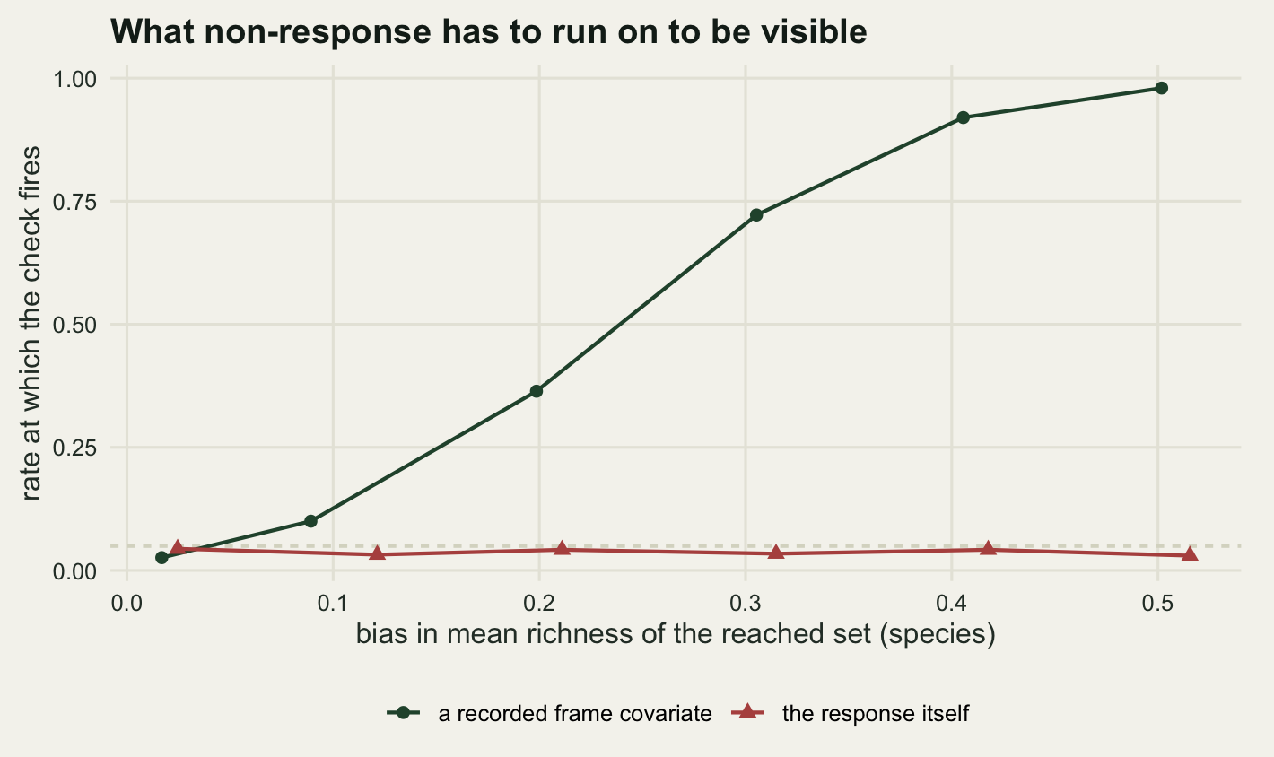
The sweep says the same thing across a range of strengths. Along the green curve the check is a good instrument, going from its null rate to near certainty as the bias grows. Along the red curve the bias grows in exactly the same way and the curve does not move. Groves and Peytcheva (2008) found across fifty-nine methodological studies that the non-response rate itself predicts bias poorly, and this is the mechanism: what matters is what the non-response ran on, and only one of the two possibilities leaves a mark on the frame. Kadmon, Farber and Danin (2004) measured the same thing in the field, where roadside accessibility rather than ecology decided which sites were surveyed.
What the check catches: selection on anything the frame recorded. What it misses: selection on the response, which is the case where the crew’s judgement was ecological. The size of the damage is measured in non-response and site substitution, including what happens when the crew fills the gap by walking to the next plot along.
Check two: is the series the product of one method?
Twenty-eight annual values from a moth network. Somewhere in the middle the bulbs were replaced, and the index dropped by an amount that has nothing to do with moths. The check scans every candidate year for a level shift, and the part that is usually got wrong is the threshold.
n_yr <- 28
k_pro <- 15L

scan_seam <- function(y, kmin = 5L) {
  n <- length(y)
  ks <- kmin:(n - kmin + 1L)
  tv <- vapply(ks, function(k) {
    a <- y[seq_len(k - 1L)]; b <- y[k:n]
    n1 <- length(a); n2 <- length(b)
    sp <- sqrt(((n1 - 1) * var(a) + (n2 - 1) * var(b)) / (n1 + n2 - 2))
    (mean(b) - mean(a)) / (sp * sqrt(1 / n1 + 1 / n2))
  }, numeric(1))
  list(k = ks, tv = tv, smax = max(abs(tv)), khat = ks[which.max(abs(tv))])
}

set.seed(41001)
null_smax <- replicate(4000, scan_seam(rnorm(n_yr))$smax)
crit_max <- unname(quantile(null_smax, 0.95))
crit_pt <- qt(0.975, n_yr - 2)
fpr_pt <- mean(null_smax > crit_pt)
n_cand <- length(scan_seam(rnorm(n_yr))$k)
print(round(c(candidate_years = n_cand, pointwise_crit = crit_pt,
              max_crit = crit_max, pointwise_false_alarm = fpr_pt), 4))
candidate_years pointwise_crit max_crit
20.0000 2.0555 2.9648
pointwise_false_alarm
0.3012 There are 20 candidate years, each giving a two-sample statistic, and the statistic that gets reported is the largest of them. Comparing that maximum against the pointwise critical value of 2.0555 flags a seam in 30.12 per cent of series that have none. The correct reference is the distribution of the maximum, whose upper five per cent point is 2.9648. Andrews (1993) derived the asymptotic distribution for this family of tests; simulating it, as here, costs a second and needs no theory. For more than one break, Killick, Fearnhead and Eckley (2012) give the segmentation machinery, and the same threshold problem returns in the choice of penalty.
step_sd <- 1.5
ramp_tot <- 2.5
ramp <- (seq_len(n_yr) - 1) / (n_yr - 1)
prof_step <- as.numeric(seq_len(n_yr) >= k_pro)

seam_run <- function(profile, mult, n_rep, seed0) {
  hit <- 0; hit_pt <- 0; loc <- integer(n_rep)
  for (r in seq_len(n_rep)) {
    set.seed(seed0 + r)
    s <- scan_seam(rnorm(n_yr) + mult * profile)
    if (s$smax > crit_max) hit <- hit + 1
    if (s$smax > crit_pt) hit_pt <- hit_pt + 1
    loc[r] <- s$khat
  }
  c(flag = hit / n_rep, flag_pointwise = hit_pt / n_rep,
    year_exact = mean(loc == k_pro), year_within_one = mean(abs(loc - k_pro) <= 1))
}
r2_step <- seam_run(prof_step, step_sd, 2000, 42000)
r2_trend <- seam_run(ramp, ramp_tot, 2000, 43000)
print(round(rbind(method_step = r2_step, smooth_trend = r2_trend), 4))
flag flag_pointwise year_exact year_within_one
method_step 0.896 0.985 0.4555 0.6975
smooth_trend 0.924 0.992 0.0670 0.1875A step of 1.5 residual standard deviations, which is what replacing a light source can easily do to a catch index, is found in 89.6 per cent of series. The scan puts the break on the right year in 45.55 per cent of them and within one year in 69.75 per cent, so a detected break a year or two away from the protocol date is not evidence against the protocol.
The second row is the problem. That series has no step at all: it is a smooth decline of 2.5 standard deviations across the twenty-eight years, the kind of thing a monitoring scheme exists to find. The scan flags a seam in 92.4 per cent of those series, slightly more often than it flags the real step, and it puts the break in the middle of the series where the two halves differ most. A seam scan run on raw index values cannot separate a method change from the finding.
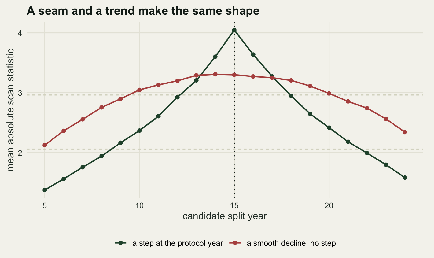
The repair is the design. The protocol names the year the equipment changed, so the test does not need twenty candidates: it needs one, and it can afford to carry a linear term for the ecology at the same time.
named_test <- function(y, detrend) {
  tt <- seq_len(n_yr)
  m <- if (detrend) lm(y ~ tt + I(tt >= k_pro)) else lm(y ~ I(tt >= k_pro))
  summary(m)$coefficients["I(tt >= k_pro)TRUE", 4]
}
named_run <- function(profile, mult, detrend, n_rep, seed0) {
  hit <- 0
  for (r in seq_len(n_rep)) {
    set.seed(seed0 + r)
    hit <- hit + (named_test(rnorm(n_yr) + mult * profile, detrend) < 0.05)
  }
  hit / n_rep
}
r2_named <- c(
  raw_step = named_run(prof_step, step_sd, FALSE, 1500, 44000),
  raw_trend = named_run(ramp, ramp_tot, FALSE, 1500, 45000),
  detrended_step = named_run(prof_step, step_sd, TRUE, 1500, 44000),
  detrended_trend = named_run(ramp, ramp_tot, TRUE, 1500, 45000))
print(round(r2_named, 4))
raw_step raw_trend detrended_step detrended_trend
0.9640 0.8913 0.4600 0.0533 Testing the named year without allowing for a trend does not fix the scan’s real problem: power of 96.4 per cent on the step and 89.13 per cent on the pure trend, so it almost always declares a seam in a series that only declined. Adding the linear term fixes the false alarm, 5.33 per cent, and the bill arrives immediately: power on the real step falls to 46 per cent, because over twenty-eight years a step in the middle and a straight line are not far apart as shapes.
What the check catches: a level shift large relative to the year-to-year variation, once its threshold accounts for the scan. What it misses: everything about attribution. A step and a real abrupt change are the same data, and only the protocol says which one you are looking at. The consequences of getting it wrong are in splicing a monitoring series, and the way to avoid the question entirely is a period when both methods run together, sized in how long a calibration overlap.
Check three: is the measurement on the grid the analysis assumes?
Seven hundred and twenty sward heights, recorded in whole centimetres. One recorder in three was working from a rule marked at five centimetre intervals and wrote down the nearest mark. Two diagnostics: the terminal digit, and the spacing of the sorted unique values.
n_ht <- 720
ht_shape <- 5.76
ht_scale <- 12 / ht_shape

record_ht <- function(x, f, coarse) {
  heaped <- runif(length(x)) < f
  out <- round(x)
  out[heaped] <- round(x[heaped] / coarse) * coarse
  out
}
gcd_pair <- function(a, b) { while (b > 0) { tmp <- b; b <- a %% b; a <- tmp }; a }
spacing_of <- function(v) Reduce(gcd_pair, as.integer(sort(unique(v)) - min(v)))
share5 <- function(v) mean(v %% 5 == 0)

set.seed(52001)
ht_obs <- record_ht(rgamma(n_ht, shape = ht_shape, scale = ht_scale), 0.30, 5)
digit_ct <- tabulate(ht_obs %% 10 + 1L, 10L)
print(rbind(digit = 0:9, count = digit_ct))
[,1] [,2] [,3] [,4] [,5] [,6] [,7] [,8] [,9] [,10]
digit 0 1 2 3 4 5 6 7 8 9
count 168 49 44 41 47 172 38 53 41 67print(round(c(share_on_multiples_of_5 = share5(ht_obs),
implied_spacing = spacing_of(ht_obs)), 4))share_on_multiples_of_5 implied_spacing
0.4722 1.0000 The table is the whole diagnostic and it takes one line. Digits 0 and 5 carry 168 and 172 of the 720 records, against the 72 an even spread across the ten digits would give, and 47.22 per cent of the file sits on a multiple of five. The spacing check returns 1, correctly: the greatest common divisor of the gaps between sorted unique values is one centimetre, because two thirds of the file is on the fine grid.
Two things have to be settled before the digit table can be used as a test. First, the digit distribution of a clean file is not uniform, because the heights are spread over only a few tens of centimetres, so a uniform chi-square is miscalibrated. Second, both statistics need a reference, and the reference can be simulated: fit a distribution to the recorded values by moments, round it to the nominal grid, and see what the statistic does.
share5_null <- function(v, n_boot) {
  m <- mean(v); s <- sd(v)
  sim <- matrix(round(rgamma(n_boot * length(v), shape = (m / s)^2,
                             scale = s^2 / m)), n_boot, length(v))
  rowMeans(sim %% 5 == 0)
}
x2_of <- function(v) {
  ct <- tabulate(v %% 10 + 1L, 10L)
  ex <- length(v) / 10
  sum((ct - ex)^2 / ex)
}
x2_null <- function(v, n_boot) {
  m <- mean(v); s <- sd(v)
  sim <- matrix(round(rgamma(n_boot * length(v), shape = (m / s)^2,
                             scale = s^2 / m)), n_boot, length(v))
  apply(sim, 1, x2_of)
}

ht_run <- function(f, coarse, n_rep, n_boot, seed0) {
  naive <- 0; targeted <- 0; omnibus <- 0; spaced <- 0
  for (r in seq_len(n_rep)) {
    set.seed(seed0 + r)
    v <- record_ht(rgamma(n_ht, shape = ht_shape, scale = ht_scale), f, coarse)
    ct <- tabulate(v %% 10 + 1L, 10L)
    if (suppressWarnings(chisq.test(ct)$p.value) < 0.05) naive <- naive + 1
    set.seed(seed0 + 500 + r)
    if (share5(v) > quantile(share5_null(v, n_boot), 0.95)) targeted <- targeted + 1
    set.seed(seed0 + 500 + r)
    if (x2_of(v) > quantile(x2_null(v, n_boot), 0.95)) omnibus <- omnibus + 1
    if (spacing_of(v) > 1) spaced <- spaced + 1
  }
  c(naive_chisq = naive / n_rep, targeted = targeted / n_rep,
    omnibus = omnibus / n_rep, spacing = spaced / n_rep)
}

ht_tab <- rbind(
  clean = ht_run(0, 5, 150, 150, 53000),
  grid5_5pct = ht_run(0.05, 5, 150, 150, 53200),
  grid5_10pct = ht_run(0.10, 5, 150, 150, 53400),
  grid2_10pct = ht_run(0.10, 2, 150, 150, 53600),
  grid2_20pct = ht_run(0.20, 2, 150, 150, 53800))
print(round(ht_tab, 4))
naive_chisq targeted omnibus spacing
clean 0.2467 0.0533 0.0600 0
grid5_5pct 0.6467 0.8533 0.3333 0
grid5_10pct 1.0000 1.0000 0.9067 0
grid2_10pct 0.7267 0.0800 0.3600 0
grid2_20pct 1.0000 0.0867 0.9600 0The naive uniform chi-square fires on 24.67 per cent of clean files, so a small p value from it means nothing on its own. Once the null is simulated the size comes right: 5.33 per cent for the targeted statistic and 6 per cent for the omnibus one.
Against the five centimetre grid the targeted statistic is the better instrument, finding a contamination of one record in twenty 85.33 per cent of the time and one record in ten 100 per cent of the time. It is also the one that goes blind. When the recorder’s rule was marked every two centimetres instead of five, the same one in ten contamination is caught in 8 per cent of files, barely above its size of 5.33 per cent, and doubling the contamination does not help: 8.67 per cent. The statistic was pointed at multiples of five, and an even grid puts almost nothing extra there.
The omnibus version, which asks only whether the digit distribution departs from what a smooth recording process would give, keeps some of the power on the five centimetre grid, 90.67 per cent, and picks up the two centimetre grid that the targeted statistic cannot see: 36 per cent at ten per cent contamination and 96 per cent at twenty. That is the usual exchange, breadth against power, and here it is worth taking, because nobody knows in advance what the rule was marked in.
The spacing check never fires in any of those rows, and that is correct behaviour rather than failure. A greatest common divisor is destroyed by one record off the grid, so it answers a narrower question: is the entire file on a coarse grid?
whole_grid <- vapply(c(10, 20, 40), function(nn) {
  ok <- 0
  for (r in 1:400) {
    set.seed(55000 + r)
    v <- round(rgamma(nn, shape = ht_shape, scale = ht_scale) / 5) * 5
    ok <- ok + (spacing_of(v) == 5)
  }
  ok / 400
}, numeric(1))
print(c(n_10 = whole_grid[1], n_20 = whole_grid[2], n_40 = whole_grid[3]))
n_10 n_20 n_40
1 1 1 For that narrower question it is close to free: with ten values already on a five centimetre grid the spacing check identifies the grid in 100 per cent of files, and at twenty and forty values in 100 and 100 per cent. Run it on each recorder separately and it becomes useful again, because the defect being chased is one recorder using one rule.
What the checks catch: heaping onto a grid whose multiples they were pointed at, and a whole file on one grid. What they miss: a grid nobody thought to test. Heitjan (1989) reviews the inference problem once the grid is known, and the price paid by an analysis that ignores it is measured in rounded and coarsened measurements and in digit preference and heaping.
Check four: do the group labels have the composition the design specified?
Sixty grassland sites, three managements, twenty sites each. The design blocked on soil depth: sites were sorted by depth into twenty blocks of three, and the three managements were allocated at random within each block. That blocking is the whole reason a plain difference of group means is admissible, and it means the design implies a distribution for the depth difference between any two arms.
n_site <- 60
arm_lv <- c("ungrazed", "grazed", "cut")
arm_eff <- c(ungrazed = 0, grazed = -1.6, cut = -0.7)
b_depth <- 1.4
b_hidden <- 0.6
sd_plot <- 2.0
true_gap <- arm_eff[["grazed"]] - arm_eff[["ungrazed"]]

set.seed(20260401)
depth <- round(rnorm(n_site), 3)
blk <- rep(seq_len(n_site / 3), each = 3)[order(order(depth))]

alloc_plan <- function(seed) {
  set.seed(seed)
  out <- character(n_site)
  for (b in unique(blk)) out[blk == b] <- sample(arm_lv)
  out
}
depth_gap <- function(lab) {
  mean(depth[lab == "grazed"]) - mean(depth[lab == "ungrazed"])
}

set.seed(46001)
null_gap <- vapply(1:4000, function(r) depth_gap(alloc_plan(200000 + r)), numeric(1))
gap_lim <- unname(quantile(null_gap, c(0.025, 0.975)))
print(round(c(sd_of_design_gap = sd(null_gap), lower = gap_lim[1],
              upper = gap_lim[2]), 4))
sd_of_design_gap lower upper
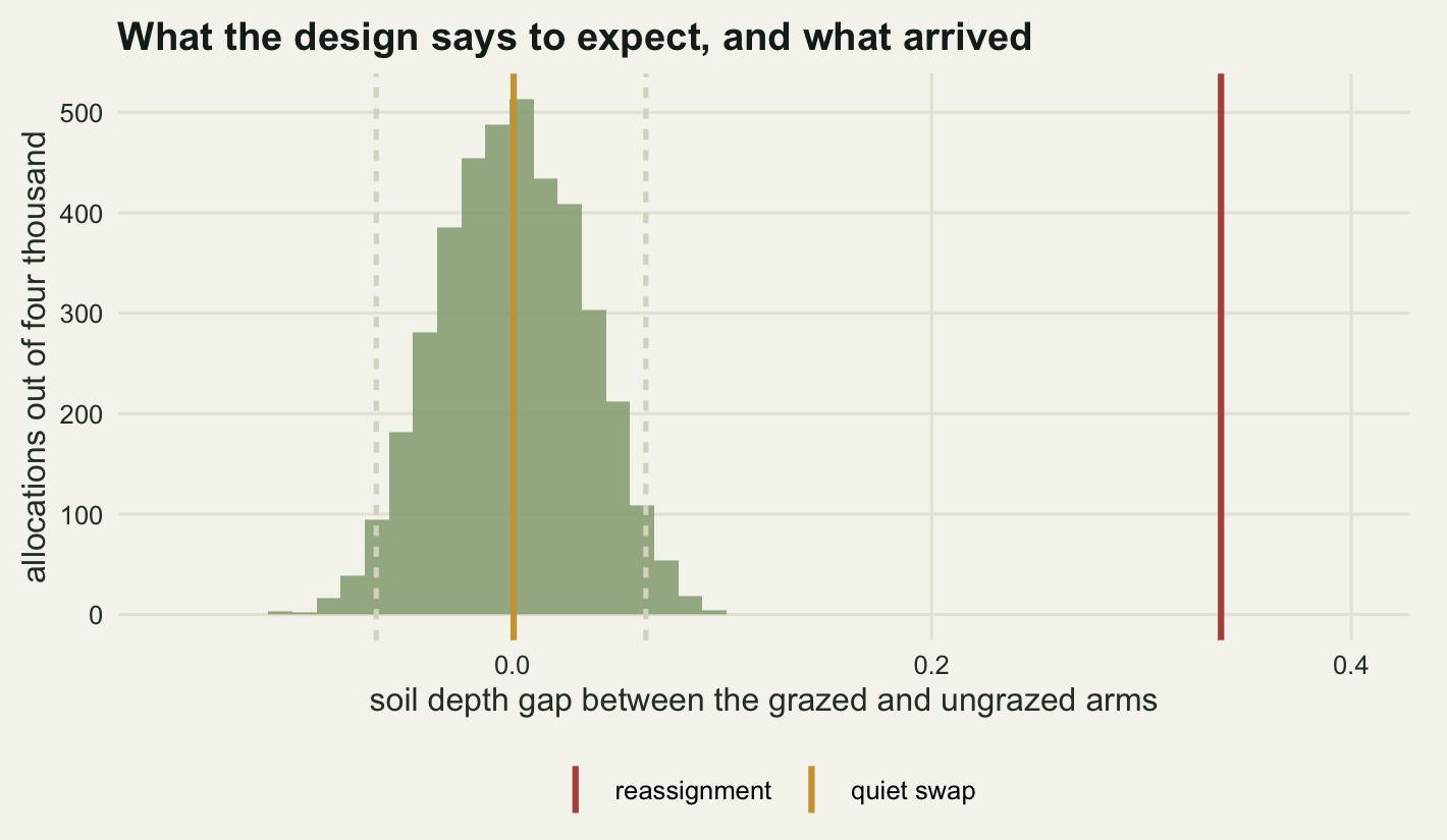
0.0339 -0.0649 0.0637 Re-running the written allocation four thousand times gives the depth gap a standard deviation of 0.0339 and a central interval from -0.0649 to 0.0637. That interval is the design speaking: under the allocation that was specified, a depth gap outside it happens five per cent of the time. Nothing in the returned data is needed to compute it.
Two ways the field can depart from that plan. In the first, sites get moved into the grazed category because the grazier had stock available, more often on the deeper soils. In the second, a botanist swaps the grazed and ungrazed member of a block on the day, on a judgement about sward quality that is nowhere in the data, and the group sizes stay exactly as planned.
alloc_rep <- function(r, mode, gg) {
  planned <- alloc_plan(80000 + r)
  set.seed(90000 + r)
  hidden <- rnorm(n_site)
  realised <- planned
  if (mode == "drift") {
    realised[runif(n_site) < plogis(-1.6 + gg * depth)] <- "grazed"
  } else if (mode == "swap") {
    for (b in unique(blk)) {
      g <- which(blk == b)
      ig <- g[planned[g] == "grazed"]
      iu <- g[planned[g] == "ungrazed"]
      if (hidden[ig] < hidden[iu]) {
        realised[ig] <- "ungrazed"
        realised[iu] <- "grazed"
      }
    }
  }
  set.seed(95000 + r)
  y <- 14 + arm_eff[realised] + b_depth * depth + b_hidden * hidden +
    rnorm(n_site, 0, sd_plot)
  sizes <- table(factor(realised, levels = arm_lv))
  gp <- depth_gap(realised)
  c(size_flag = any(sizes != n_site / 3),
    t_flag = t.test(depth[realised == "grazed"],
                    depth[realised == "ungrazed"])$p.value < 0.05,
    design_flag = gp < gap_lim[1] || gp > gap_lim[2],
    est = mean(y[realised == "grazed"]) - mean(y[realised == "ungrazed"]),
    gap = gp, n_grazed = sizes[["grazed"]], n_ungrazed = sizes[["ungrazed"]])
}
summ4 <- function(mode, gg) {
  M <- t(vapply(1:1200, alloc_rep, numeric(7), mode = mode, gg = gg))
  c(size_flag = mean(M[, "size_flag"]), t_flag = mean(M[, "t_flag"]),
    design_flag = mean(M[, "design_flag"]), gap = mean(M[, "gap"]),
    bias = mean(M[, "est"]) - true_gap, n_grazed = mean(M[, "n_grazed"]),
    n_ungrazed = mean(M[, "n_ungrazed"]))
}
r4_ok <- summ4("none", 0)
r4_drift <- summ4("drift", 1.2)
r4_swap <- summ4("swap", 0)
print(round(rbind(as_designed = r4_ok, reassignment = r4_drift,
                  quiet_swap = r4_swap), 4))
size_flag t_flag design_flag gap bias n_grazed n_ungrazed
as_designed 0 0.0000 0.0550 -0.0009 -0.0091 20.0000 20.0000
reassignment 1 0.0608 0.9750 0.3379 0.4562 27.9142 16.0292
quiet_swap 0 0.0000 0.0525 0.0006 0.7119 20.0000 20.0000When the field followed the plan the contrast is unbiased: a mean error of -0.0091 units on a true difference of -1.6. The design reference sits at its nominal rate, 5.5 per cent, while the t test never fires at all, the first sign of the mismatch that the reassignment row makes explicit.
Under reassignment the arms end up at 27.91 and 16.03 sites on average instead of 20 each, so the size check fires in 100 per cent of realisations. The depth gap averages 0.3379, and the estimated grazing effect is 0.4562 units out, 0.228 of a residual standard deviation. Here the two balance checks part company. A two-sample test on depth, the one that gets run, fires 6.08 per cent of the time. The same gap read against the design’s own randomisation distribution fires 97.5 per cent of the time. Same data, same statistic, different reference, and the difference is the whole point: a t test asks whether the gap is large compared with the variation between sites, and the design already promised something far tighter than that. Senn (1994) argued that significance tests on baseline covariates are the wrong instrument in a randomised trial; Imai, King and Stuart (2008) make the same case and point at the randomisation distribution as the reference that means something.
The quiet swap is where all three checks stop. The sizes are exactly as planned, so the size check fires 0 per cent of the time. The swap ignores depth, so the depth gap is 0.0006 and the design reference fires 5.25 per cent, its null rate. And the bias is 0.7119 units, 1.561 times the bias in the case every check caught.
One more check belongs here and needs no simulation, because it is arithmetic. A unit must appear in exactly one group, exactly once.
site_id <- sprintf("S%02d", seq_len(n_site))
alloc_tab <- data.frame(site = site_id, arm = alloc_plan(80001),
                        stringsAsFactors = FALSE)
wrong_arm <- setdiff(arm_lv, alloc_tab$arm[alloc_tab$site == "S07"])[1]
alloc_tab <- rbind(alloc_tab,
                   data.frame(site = "S07", arm = wrong_arm),
                   alloc_tab[alloc_tab$site == "S22", ])
arms_per_site <- tapply(alloc_tab$arm, alloc_tab$site, function(a) length(unique(a)))
rows_per_site <- table(alloc_tab$site)
print(c(rows = nrow(alloc_tab), sites = length(rows_per_site),
        in_two_arms = sum(arms_per_site > 1),
        listed_twice = sum(rows_per_site > 1)))
rows sites in_two_arms listed_twice
62 60 1 2 print(names(rows_per_site)[rows_per_site > 1])[1] "S07" "S22"Two lines, and they find both planted faults: 1 site listed under two managements and 2 sites listed more than once. This check has no power curve because it has no null; either the table has the shape the design specified or it does not. It is also the one most often skipped, because a duplicated row does not break anything downstream. It quietly reweights the unit.
What the checks catch: any departure that shows up in the recorded columns, provided the reference is the design’s own randomisation distribution rather than a t test. What they miss: a reallocation on a criterion nobody wrote down, which is the common case, since the field decision that overrides a plan is usually a judgement rather than a number. When the outcome itself is what drove the group, the damage looks like the effect measured in baseline selection and the return to mean.
Check five: are the identifiers stable over the series?
Twenty years of counts for sixty taxa, two eras of ten years. Some taxa arrive, some disappear, and six of them keep their organism and change their code at the era boundary: a revision, a new recording app, a site register renumbered. Each renamed taxon becomes two labels, one that stops at year ten and one that starts at year eleven.
n_tax <- 60
n_year <- 20
late <- seq_len(n_year) > 10

set.seed(20260501)
a_tax <- rnorm(n_tax, log(2.6), 1.4)
b_tax <- rnorm(n_tax, 0, 0.30)
lam_tax <- exp(outer(a_tax, rep(1, n_year)) +
                 outer(b_tax, seq_len(n_year) - mean(seq_len(n_year))))
tax_ord <- order(a_tax)
who_mid <- tax_ord[28:33]
who_rare <- tax_ord[1:6]

churn_stat <- function(M) {
  tot <- rowSums(M)
  in1 <- rowSums(M[, !late, drop = FALSE])
  in2 <- rowSums(M[, late, drop = FALSE])
  single <- (in1 == 0 | in2 == 0) & tot > 0
  c(n_single = sum(single), share = sum(tot[single]) / sum(tot))
}
draw_counts <- function(seed) {
  set.seed(seed)
  matrix(rpois(length(lam_tax), lam_tax), n_tax, n_year)
}
split_labels <- function(M, who) {
  keep <- setdiff(seq_len(n_tax), who)
  old_rows <- M[who, , drop = FALSE]; old_rows[, late] <- 0
  new_rows <- M[who, , drop = FALSE]; new_rows[, !late] <- 0
  rbind(M[keep, , drop = FALSE], old_rows, new_rows)
}
real_turnover <- function(M, who, seed) {
  keep <- setdiff(seq_len(n_tax), who)
  lost <- M[who, , drop = FALSE]; lost[, late] <- 0
  set.seed(seed)
  colonists <- matrix(rpois(length(who) * n_year, lam_tax[who, ]),
                      length(who), n_year)
  colonists[, !late] <- 0
  rbind(M[keep, , drop = FALSE], lost, colonists)
}

null5 <- t(vapply(1:1200, function(r) churn_stat(draw_counts(300000 + r)),
                  numeric(2)))
q_n <- unname(quantile(null5[, "n_single"], 0.95))
q_s <- unname(quantile(null5[, "share"], 0.95))
print(round(c(mean_single_labels = mean(null5[, "n_single"]), upper_95 = q_n,
              mean_share = mean(null5[, "share"]), upper_95_share = q_s), 5))
mean_single_labels upper_95 mean_share upper_95_share
2.86667 5.00000 0.00170 0.00444 With no renaming at all, 2.867 labels on average are confined to one era, purely from colonisation, loss and Poisson zeros among the rare taxa, and 0.17 per cent of the recorded individuals sit on them. Those are the numbers a stable code list produces, and they are the reference.
arm5 <- function(build, who, seed_off) {
  M <- t(vapply(1:1200, function(r) {
    cnt <- draw_counts(300000 + r)
    churn_stat(if (is.null(seed_off)) build(cnt, who)
               else build(cnt, who, seed_off + r))
  }, numeric(2)))
  c(n_single = mean(M[, "n_single"]), flag_count = mean(M[, "n_single"] > q_n),
    share = mean(M[, "share"]), flag_share = mean(M[, "share"] > q_s))
}
r5_mid <- arm5(split_labels, who_mid, NULL)
r5_rare <- arm5(split_labels, who_rare, NULL)
r5_turn <- arm5(real_turnover, who_mid, 400000)
print(round(rbind(renamed_mid = r5_mid, renamed_rare = r5_rare,
                  genuine_turnover = r5_turn), 5))
n_single flag_count share flag_share
renamed_mid 14.86500 1 0.00990 1.00000
renamed_rare 10.65167 1 0.00275 0.24417
genuine_turnover 14.86583 1 0.00990 1.00000print(round(c(mean_abundance_mid = mean(exp(a_tax[who_mid])),
mean_abundance_rare = mean(exp(a_tax[who_rare]))), 4)) mean_abundance_mid mean_abundance_rare
2.4353 0.2943 Renaming six taxa of middling abundance takes the single-era label count to 14.865 against an upper five per cent point of 5, so the count fires every time. The abundance share goes to 0.99 per cent and fires every time as well. Renaming the six rarest taxa instead still moves the count to 10.652, still flagged in 100 per cent of series, but the abundance share only reaches 0.2749 per cent and clears the reference in 24.42 per cent. That is the division of labour worth keeping: the count says something happened, the share says whether it can move a total.
The third row is why the count alone is not a finding. There the six taxa genuinely died out after year ten and six genuine colonists arrived, drawn from the same abundance distribution. No label is wrong. The count is 14.866 against 14.865 for the renaming, the two differing by 0.0008 of a label, because both constructions create twelve one-era labels. The abundance share is 0.9896 per cent against 0.99 per cent, and both fire at 100 per cent. The two worlds are the same table.
What the check catches: churn in the identifier column, cheaply and with certainty. What it misses: the reason for the churn. Sorting the two apart needs the code list with its dates, and what it costs when nobody sorts them is in taxonomic revision and species trends, while the price of the standard repair is in the price of harmonising a species list.
The five checks side by side
gate_lab <- c("1  the sampled set", "2  one method", "3  the measurement grid",
              "4  the group labels", "5  the identifiers")
gate_case <- c("selection on the response, same bias",
               "a smooth decline and no step",
               "a two centimetre grid, same fraction",
               "a size-preserving swap on a hidden criterion",
               "genuine turnover of the same size")
gate_tab <- data.frame(
  check = gate_lab,
  companion = gate_case,
  aimed_at = c(r1_seen[["flag"]], r2_step[["flag"]],
               ht_tab["grid5_10pct", "targeted"], r4_drift[["design_flag"]],
               r5_mid[["flag_share"]]),
  companion_rate = c(r1_hidden[["flag"]], r2_trend[["flag"]],
                     ht_tab["grid2_10pct", "targeted"],
                     r4_swap[["design_flag"]], r5_turn[["flag_share"]]))
gate_tab$separation <- gate_tab$aimed_at - gate_tab$companion_rate
print(gate_tab[, c("check", "aimed_at", "companion_rate", "separation")],
      row.names = FALSE, digits = 3)
check aimed_at companion_rate separation
1 the sampled set 0.897 0.0507 0.846
2 one method 0.896 0.9240 -0.028
3 the measurement grid 1.000 0.0800 0.920
4 the group labels 0.975 0.0525 0.923
5 the identifiers 1.000 1.0000 0.000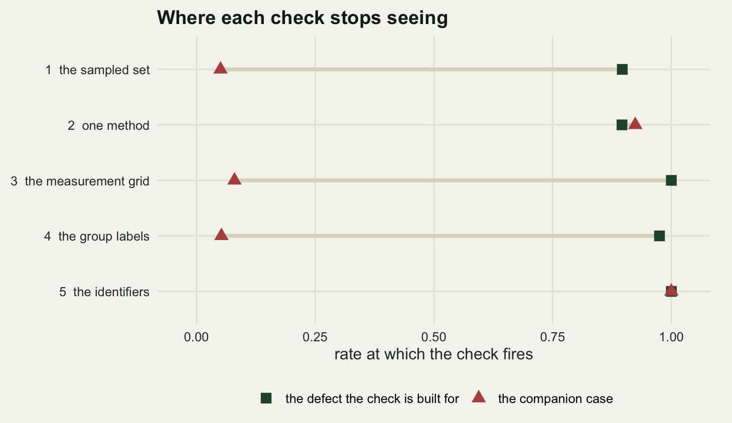
Three of the five separate their two cases by at least 0.846, which makes them worth the minute they take. The other two do not, and they fail in different ways. Check two fires 92.4 per cent of the time on a series whose only feature is a real decline, against 89.6 per cent on the method step, so a positive result from it is not evidence of a seam until the protocol date is brought in. Check five fires at 100 per cent on renaming and 100 per cent on genuine turnover, a separation of 0, which is another way of saying the statistic is a prompt rather than a diagnosis.
What none of these checks can see
Every one of the five compares the data with a written record of something: the frame and the list of cells drawn, the protocol with its dates, the recording precision on the field card, the allocation and its blocking, the code list with the year each code changed. The computation is short in all five cases. What is doing the work is the document.
That has an uncomfortable corollary. Remove the document and the check does not get weaker, it stops existing. There is no reference distribution for the depth gap without the allocation, because the interval in check four came from re-running the written plan and nothing in the returned table can produce it. There is no seam test at a named year without a protocol date, and check two showed what happens when you look for the year in the data instead. There is no comparison of reached with unreached cells if only the reached ones were kept, which is the ordinary state of a returned dataset. The five diagnostics here are cheap because the expensive part was done by somebody else, years earlier, in a text file.
Where the record is missing, the honest report is not that the check passed. It is that the check could not be run, and the assumption it would have tested is still an assumption. Isaac and colleagues (2014) made this argument for opportunistic recording, where the reason a record exists is itself unrecorded; Reichman, Jones and Schildhauer (2011) made the general version for ecological data. Both come to the same place. Writing down the frame, the protocol dates, the recording precision, the allocation and the code list is a small task at the time and the only thing that makes any of these five checks possible afterwards. The check is a documentation question first and a statistical one second.
References
Groves RM, Peytcheva E 2008 Public Opinion Quarterly 72(2):167-189 (10.1093/poq/nfn011)
Kadmon R, Farber O, Danin A 2004 Ecological Applications 14(2):401-413 (10.1890/02-5364)
Andrews DWK 1993 Econometrica 61(4):821-856 (10.2307/2951764)
Killick R, Fearnhead P, Eckley IA 2012 Journal of the American Statistical Association 107(500):1590-1598 (10.1080/01621459.2012.737745)
Isaac NJB, van Strien AJ, August TA, de Zeeuw MP, Roy DB 2014 Methods in Ecology and Evolution 5(10):1052-1060 (10.1111/2041-210X.12254)
Heitjan DF 1989 Statistical Science 4(2):164-179 (10.1214/ss/1177012601)
Senn S 1994 Statistics in Medicine 13(17):1715-1726 (10.1002/sim.4780131703)
Imai K, King G, Stuart EA 2008 Journal of the Royal Statistical Society Series A 171(2):481-502 (10.1111/j.1467-985X.2007.00527.x)
Reichman OJ, Jones MB, Schildhauer MP 2011 Science 331(6018):703-705 (10.1126/science.1197962)