Instrument drift, run order and check standards

Samples run through an analyser in treatment order turn instrument drift into an effect. Measuring in R what check standards fix and what run order does.

Thirty soil extracts from a nitrogen addition experiment are waiting in a fridge: fifteen from control plots and fifteen from plots that have received fertiliser for three seasons. They go through a flow autoanalyser for nitrate in one afternoon. The rack is loaded the way the bags came back from the field, control plots first and then the addition plots, because that is how the sample sheet was typed and it makes the printout easy to read. The instrument is warm, the reagents are fresh at the start, and over a few hours the response creeps: a lamp ages, a reagent loses strength, a tube stretches. A reading taken late in the run is a few per cent different from the same extract read early.

When the rack is sorted by treatment, that creep is not noise. Everything read late is fertilised, so every unit of drift lands in the treatment difference. The usual laboratory defence is a check standard, a solution of known concentration read every five or ten samples, with the samples between two standards corrected by linear interpolation. Metabolomics made this routine: Dunn and colleagues describe pooled quality control samples spaced through a run and a fitted drift curve subtracted from every injection. The defence that costs nothing is older. Box, Hunter and Hunter treat the order of runs as something to randomise because an unrandomised order lets any trend in time impersonate a factor, and Hurlbert’s account of pseudoreplication calls the spatial form of the same failure segregation: units of one treatment grouped together instead of interspersed. Leek and colleagues showed how often processing batches confound biological comparisons in genomics. None of this is new, and this post is a demonstration of those sources on a soil laboratory run, not a discovery.

The site already has several relatives. Depth sensor drift and the dive count corrects a drifting pressure sensor from the readings taken while a seal floats at the surface, a known reference state the animal keeps returning to; nothing there is confounded with a treatment. Values below the detection limit shows an improving laboratory manufacturing a decline in a monitoring series through its falling limit, and checking your data against the design scans a series for the year a method changed. Those are trends across years. Here the trend lasts one afternoon, and the design choice that decides whether it matters is the order of the rack. The mechanism that keeps the standards from finishing the job turns out to be the one in pseudoreplication and false positives: an error shared by several samples of the same group.

The post does four things. It derives the false positive rate of a sorted run from a noncentral t distribution and checks it against simulation. It measures what check standards every ten or five samples leave behind, and finds that the remainder is not drift but the standards’ own reading error, so its size is set by how precisely a standard is read. It turns the whole run sheet into a covariance calculation that predicts the rate for any order and any standard spacing, and sweeps drift size with it. Finally it compares power, including run position fitted as a smooth in a randomised run.

library(ggplot2)
library(patchwork)
library(mgcv)

te_paper  <- "#f5f4ee"
te_ink    <- "#16241d"
te_body   <- "#2c3a31"
te_forest <- "#275139"
te_rust   <- "#b5534e"
te_gold   <- "#c9b458"
te_line   <- "#dad9ca"

theme_datasheet <- function() {
  theme_minimal(base_size = 12) +
    theme(plot.background  = element_rect(fill = te_paper, colour = NA),
          panel.background = element_rect(fill = te_paper, colour = NA),
          panel.grid.major = element_line(colour = te_line, linewidth = 0.3),
          panel.grid.minor = element_blank(),
          text             = element_text(colour = te_body),
          plot.title       = element_text(colour = te_ink, face = "bold"),
          plot.subtitle    = element_text(colour = te_body),
          axis.text        = element_text(colour = te_body))
}

The run and its drift

Every quantity below is on the natural log scale, so a difference of 0.1 is close to a ten per cent ratio and a correction by a standard is a division. The design constants were fixed before any simulation was run. Field variation between plots has a standard deviation of 0.15, an assumed spread for extractable nitrate among plots of one treatment. Each reading carries an analytical error of 3 per cent (0.03), and a check standard is read with that same error. The drift is a straight creep of 0.4 per cent per position plus a random walk whose steps have a standard deviation of 1 per cent. Standards, when used, sit at the start of the run, after every k samples and at the end, and they take positions in the run like samples do, so a run with standards is longer and drifts further. The test is the two-sample t test on log values that the analysis would use anyway, and a true effect for power is a ten per cent increase.

n_per    <- 15
n_smp    <- 2 * n_per
sd_field <- 0.15
sd_an    <- 0.03
lin_main <- 0.004
rw_main  <- 0.01
eff_10   <- log(1.10)
n_run    <- 4000
t_crit   <- qt(0.975, n_smp - 2)

run_layout <- function(k_std) {
  if (k_std == 0) return(list(slot = seq_len(n_smp), std = integer(0), m = n_smp))
  ids <- 0L
  for (i in seq_len(n_smp)) {
    ids <- c(ids, i)
    if (i %% k_std == 0) ids <- c(ids, 0L)
  }
  if (tail(ids, 1) != 0L) ids <- c(ids, 0L)
  list(slot = which(ids > 0), std = which(ids == 0), m = length(ids))
}

interp_weights <- function(lay) {
  n_std <- length(lay$std)
  if (n_std == 0) return(matrix(0, n_smp, 0))
  sapply(seq_len(n_std), function(j) {
    unit <- numeric(n_std)
    unit[j] <- 1
    approx(lay$std, unit, xout = lay$slot, rule = 2)$y
  })
}

treat_slots <- function(order_name, n_rep) {
  one_sheet <- switch(order_name,
                      sorted      = rep(c(FALSE, TRUE), each = n_per),
                      alternating = rep(c(FALSE, TRUE), times = n_per))
  if (!is.null(one_sheet)) return(matrix(one_sheet, n_rep, n_smp, byrow = TRUE))
  t(apply(matrix(runif(n_rep * n_smp), n_rep), 1, function(u) rank(u) > n_per))
}

row_tstat <- function(y, g) {
  m1 <- rowSums(y * g) / n_per
  m0 <- rowSums(y * !g) / n_per
  ss <- rowSums((y - ifelse(g, m1, m0))^2)
  (m1 - m0) / sqrt(ss / (n_smp - 2) * 2 / n_per)
}

sim_runs <- function(order_name, k_std, lin, rw, eff = 0, n_rep = n_run,
                     sd_std = sd_an, keep = FALSE) {
  lay    <- run_layout(k_std)
  g      <- treat_slots(order_name, n_rep)
  drift  <- t(apply(matrix(rnorm(n_rep * lay$m, lin, rw), n_rep), 1, cumsum))
  err_sd <- rep(sd_an, lay$m)
  err_sd[lay$std] <- sd_std
  meas   <- drift + sweep(matrix(rnorm(n_rep * lay$m), n_rep), 2, err_sd, "*")
  y <- matrix(rnorm(n_rep * n_smp, 0, sd_field), n_rep) + eff * g +
       meas[, lay$slot, drop = FALSE]
  if (k_std > 0) {
    y <- y - meas[, lay$std, drop = FALSE] %*% t(interp_weights(lay))
  }
  tt <- row_tstat(y, g)
  if (keep) return(list(y = y, g = g, t = tt))
  mean(abs(tt) > t_crit)
}

mc_se <- function(p, n) sqrt(p * (1 - p) / n)

Each simulated run is one row of a matrix, so thousands of runs cost a fraction of a second. The run sheet is a logical vector over the thirty sample slots, true where the slot holds an addition plot. A sorted sheet is fifteen false then fifteen true, an alternating sheet swaps at every slot, and a randomised sheet is a fresh permutation for every run. The rate of a design is the share of 4000 simulated runs in which the t test rejects at five per cent; its Monte Carlo standard error at a rate of 0.05 is 0.0034.

A sorted run turns drift into a treatment effect

Start with the straight creep alone. In a sorted run of thirty samples the addition plots sit, on average, fifteen positions after the controls, so the drift adds a fixed shift of fifteen times the creep to the treatment difference. The t statistic is then a noncentral t: its numerator is the true shift plus the usual sampling noise, and its noncentrality is the shift divided by the standard error of the difference. One small correction is needed for exactness. The creep also spreads the samples within each group, which inflates the pooled variance the test divides by, and that inflation is a deterministic sum of squares.

shift_lin   <- lin_main * n_per
sd_sample   <- sqrt(sd_field^2 + sd_an^2)
se_nominal  <- sd_sample * sqrt(2 / n_per)
trend_ss    <- 2 * lin_main^2 * sum((seq_len(n_per) - mean(seq_len(n_per)))^2)
se_expected <- sqrt(sd_sample^2 + trend_ss / (n_smp - 2)) * sqrt(2 / n_per)
ncp_lin     <- shift_lin / se_nominal
q_lin       <- t_crit * se_expected / se_nominal
rate_closed <- 1 - pt(q_lin, n_smp - 2, ncp_lin) + pt(-q_lin, n_smp - 2, ncp_lin)

n_big <- 40000
set.seed(3101)
rate_lin_sim <- sim_runs("sorted", 0, lin_main, 0, n_rep = n_big)
gap_lin_se   <- (rate_closed - rate_lin_sim) / mc_se(rate_lin_sim, n_big)
rate_rw_sim  <- sim_runs("sorted", 0, lin_main, rw_main)

A creep of 0.4 per cent per position shifts the log difference by 0.060, against a standard error of 0.0559. The noncentrality is 1.074, and the noncentral t gives a rejection rate of 0.1761 for a test that should reject in five per cent of runs. Over 40000 simulated sorted runs with the creep alone, the rate was 0.1766, 0.3 Monte Carlo standard errors from the formula. Nothing about this rate needs a simulation; it is a line of pt().

Adding the random walk on top brings the simulated rate to 0.2110. The walk does not bias the difference on average, because it wanders up as often as down, but in a sorted run the two halves of one walk are compared with each other, and the variance of that comparison is not in the standard error the test uses.

set.seed(3100)
lay_five  <- run_layout(5)
drift_one <- cumsum(rnorm(lay_five$m, lin_main, rw_main))
read_one  <- drift_one + rnorm(lay_five$m, 0, sd_an)
group_one <- factor(rep(c("control", "N addition"), each = n_per),
                    levels = c("control", "N addition"))
field_one <- rnorm(n_smp, 0, sd_field)
raw_smp   <- field_one + read_one[lay_five$slot]
corr_smp  <- raw_smp - as.vector(interp_weights(lay_five) %*% read_one[lay_five$std])

smp_df <- data.frame(pos = lay_five$slot, raw = raw_smp, corrected = corr_smp,
                     group = group_one)
std_df <- data.frame(pos = lay_five$std, reading = read_one[lay_five$std])
drift_df <- data.frame(pos = seq_len(lay_five$m), drift = drift_one)
grp_cols <- c("control" = te_forest, "N addition" = te_rust)

p_raw <- ggplot() +
  geom_line(data = drift_df, aes(pos, drift), colour = te_ink, linewidth = 0.7) +
  geom_point(data = smp_df, aes(pos, raw, colour = group), size = 2.3) +
  geom_point(data = std_df, aes(pos, reading), shape = 23, size = 2.8,
             fill = te_gold, colour = te_ink) +
  scale_colour_manual(values = grp_cols, name = NULL) +
  labs(x = "run position", y = "log reading, relative to truth",
       title = "As read", subtitle = "line: true drift; diamonds: check standards") +
  theme_datasheet() +
  theme(legend.position = "bottom")

p_corr <- ggplot(smp_df, aes(pos, corrected, colour = group)) +
  geom_hline(yintercept = 0, colour = te_body, linetype = "dashed", linewidth = 0.4) +
  geom_point(size = 2.3) +
  scale_colour_manual(values = grp_cols, name = NULL) +
  labs(x = "run position", y = "log reading after correction",
       title = "After standards", subtitle = "no true treatment effect in this run") +
  theme_datasheet() +
  theme(legend.position = "bottom")

p_raw + p_corr + plot_layout(guides = "collect") +
  plot_annotation(theme = theme_datasheet() + theme(legend.position = "bottom"))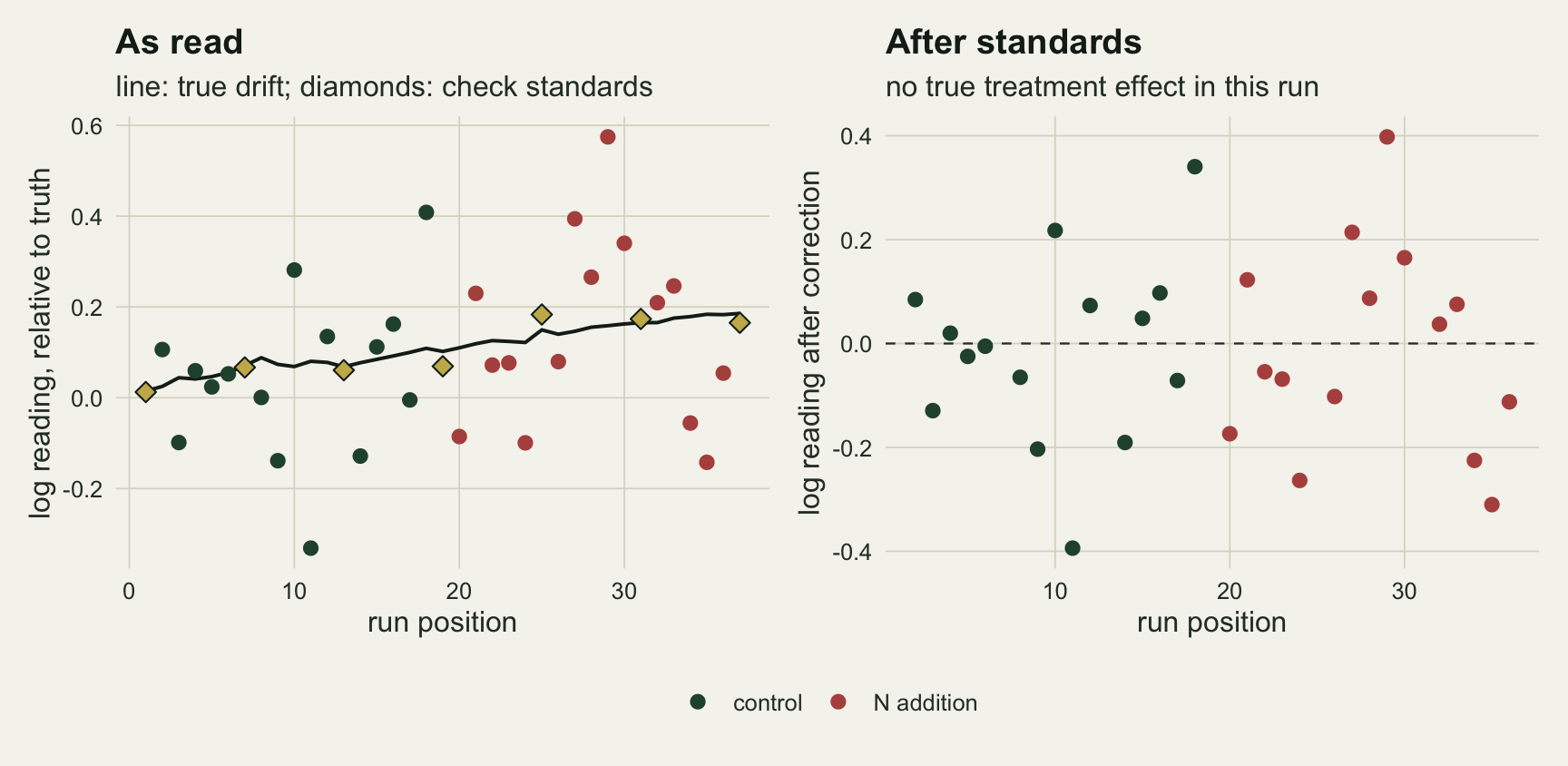

Figure 1: One simulated sorted run with a check standard every five samples: raw readings with the true drift (left), and the same samples after interpolated correction (right).

What the check standards leave behind

The next chunk runs every combination of three run orders and three standard spacings under the full drift, once with no effect and once with a ten per cent effect.

set.seed(3102)
grid_res <- expand.grid(order = c("sorted", "alternating", "random"),
                        k_std = c(0, 10, 5), stringsAsFactors = FALSE)
grid_res$type1 <- mapply(function(o, k) sim_runs(o, k, lin_main, rw_main),
                         grid_res$order, grid_res$k_std)
grid_res$power <- mapply(function(o, k) sim_runs(o, k, lin_main, rw_main, eff = eff_10),
                         grid_res$order, grid_res$k_std)

res_of <- function(o, k, what) grid_res[grid_res$order == o & grid_res$k_std == k, what]
other_t1 <- grid_res$type1[grid_res$order != "sorted"]

n_zero    <- 20000
zero_5    <- sim_runs("sorted", 5, 0, 0, n_rep = n_zero)
zero_10   <- sim_runs("sorted", 10, 0, 0, n_rep = n_zero)
zero_alt5 <- sim_runs("alternating", 5, 0, 0, n_rep = n_zero)

With no standards the sorted run rejected in 0.2023 of runs. Standards every ten samples brought that to 0.0725 and every five to 0.0663. The alternating and randomised orders, with or without standards, stayed between 0.0408 and 0.0550. The run order did in one step what standards read to 3 per cent did not finish.

The obvious reading is that interpolation between standards cannot follow a random walk exactly, so some drift survives between them. That reading is wrong here, and a run with no drift at all shows it. With the creep and the walk both set to zero, a sorted run with standards every five samples still rejected in 0.0630 of 20000 runs, and with standards every ten in 0.0685, against a Monte Carlo standard error of 0.0015. An alternating run with the same standards gave 0.0469.

The excess comes from the standards themselves. Each standard reading carries its own analytical error, and the interpolated correction passes that error to every sample between it and its neighbours. In a sorted run those neighbours belong to the same group, so one unlucky standard moves several control readings together, or several addition readings together. That is an error shared within a group, and the t test counts the fifteen samples as fifteen independent pieces of information, which is the pseudoreplication mistake in laboratory form. Standards every ten samples are worse than every five because each reading is shared by more samples. In an alternating run the same shared error falls on both groups equally and cancels from the difference.

grid_long <- rbind(
  data.frame(grid_res[, c("order", "k_std")], metric = "false positive rate",
             rate = grid_res$type1),
  data.frame(grid_res[, c("order", "k_std")], metric = "power at +10 per cent",
             rate = grid_res$power))
grid_long$se <- mc_se(grid_long$rate, n_run)
grid_long$standards <- factor(ifelse(grid_long$k_std == 0, "none",
                                     paste("every", grid_long$k_std)),
                              levels = c("none", "every 10", "every 5"))
grid_long$order <- factor(grid_long$order, levels = c("sorted", "alternating", "random"))
ref_df <- data.frame(metric = "false positive rate", yint = 0.05)

ggplot(grid_long, aes(order, rate, colour = standards)) +
  geom_hline(data = ref_df, aes(yintercept = yint), linetype = "dashed",
             colour = te_body, linewidth = 0.4) +
  geom_errorbar(aes(ymin = rate - 2 * se, ymax = rate + 2 * se),
                width = 0.15, linewidth = 0.5,
                position = position_dodge(width = 0.5)) +
  geom_point(size = 2.6, position = position_dodge(width = 0.5)) +
  facet_wrap(~ metric, scales = "free_y") +
  scale_colour_manual(values = c("none" = te_rust, "every 10" = te_gold,
                                 "every 5" = te_forest),
                      name = "check standards") +
  labs(x = "run order", y = "share of runs rejecting",
       title = "Order removes the confounding; imprecise standards leave some behind",
       subtitle = "drift 0.4 per cent per position plus random walk SD 1 per cent") +
  theme_datasheet() +
  theme(legend.position = "bottom")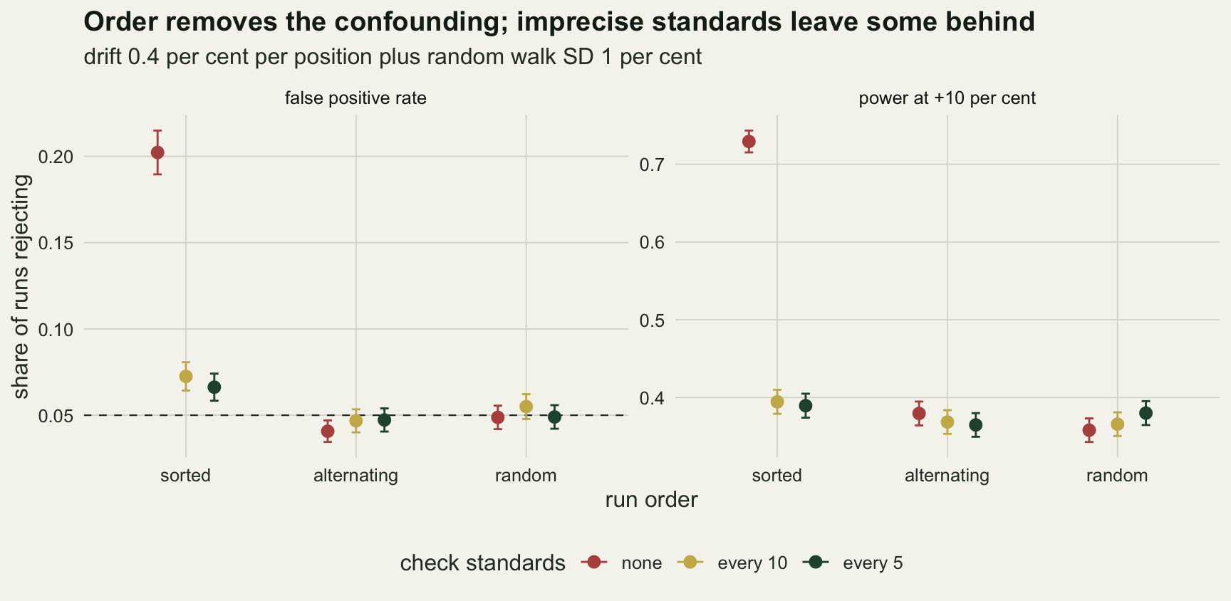

Figure 2: Rejection rates under the null (left) and at a ten per cent true effect (right) for three run orders and three standard spacings, with the full drift. Bars are two Monte Carlo standard errors.

The sorted run’s power of 0.7292 is not power. It is drift in the same direction as the effect, and a drift running the other way would have hidden a real increase just as readily.

The run sheet is a covariance calculation

Everything in this model is linear and Gaussian. A corrected reading is the field value, plus the drift at its position, plus its own error, minus a weighted sum of the standard readings, and each of those is a known linear function of independent normal variables. The random walk has the covariance of a Brownian path, the standard deviation of a step squared times the smaller of two positions. So the mean and variance of the treatment difference for any run sheet can be written down, and so can the expected pooled variance the t test uses. Plugging both into a noncentral t gives a predicted false positive rate for a sheet before a single sample is read.

predict_rate <- function(g, k_std, lin, rw, eff = 0, sd_std = sd_an) {
  lay   <- run_layout(k_std)
  w_int <- interp_weights(lay)
  m     <- lay$m
  cmat  <- matrix(0, n_smp, m)
  cmat[cbind(seq_len(n_smp), lay$slot)] <- 1
  if (k_std > 0) cmat[, lay$std] <- cmat[, lay$std] - w_int
  mu    <- eff * g + lin * as.vector(cmat %*% seq_len(m))
  sigma <- diag(sd_field^2 + sd_an^2, n_smp) + sd_std^2 * w_int %*% t(w_int) +
           rw^2 * cmat %*% outer(seq_len(m), seq_len(m), pmin) %*% t(cmat)
  a_vec  <- ifelse(g, 1, -1) / n_per
  mean_d <- sum(a_vec * mu)
  var_d  <- drop(t(a_vec) %*% sigma %*% a_vec)
  q_mat  <- diag(n_smp) - (outer(g, g, "&") + outer(!g, !g, "&")) / n_per
  s2     <- (sum(diag(q_mat %*% sigma)) + drop(t(mu) %*% q_mat %*% mu)) / (n_smp - 2)
  q_val  <- t_crit * sqrt(s2 * 2 / n_per) / sqrt(var_d)
  ncp    <- mean_d / sqrt(var_d)
  c(rate = 1 - pt(q_val, n_smp - 2, ncp) + pt(-q_val, n_smp - 2, ncp),
    shift = mean_d, sd_diff = sqrt(var_d), se_test = sqrt(s2 * 2 / n_per))
}

sheet_sorted <- rep(c(FALSE, TRUE), each = n_per)
sheet_alt    <- rep(c(FALSE, TRUE), times = n_per)

fixed_rows <- grid_res$order != "random"
grid_res$predicted <- NA_real_
grid_res$predicted[fixed_rows] <- mapply(function(o, k) {
  sheet <- if (o == "sorted") sheet_sorted else sheet_alt
  predict_rate(sheet, k, lin_main, rw_main)[["rate"]]
}, grid_res$order[fixed_rows], grid_res$k_std[fixed_rows])
gap_grid <- abs(grid_res$predicted - grid_res$type1)[fixed_rows] /
            mc_se(grid_res$type1[fixed_rows], n_run)

zero_pred5  <- predict_rate(sheet_sorted, 5, 0, 0)
zero_pred10 <- predict_rate(sheet_sorted, 10, 0, 0)

std_sweep <- expand.grid(sd_std = c(0.01, 0.02, 0.03, 0.05), k_std = c(10, 5))
std_sweep$sorted <- mapply(function(s, k) predict_rate(sheet_sorted, k, 0, 0, sd_std = s)[["rate"]],
                           std_sweep$sd_std, std_sweep$k_std)
sweep_of <- function(s, k) std_sweep$sorted[std_sweep$sd_std == s & std_sweep$k_std == k]
full_std <- sapply(c(0.01, 0.03), function(s) sapply(c(10, 5), function(k)
  predict_rate(sheet_sorted, k, lin_main, rw_main, sd_std = s)[["rate"]]))

set.seed(3103)
n_sheet     <- 2000
sheets      <- replicate(n_sheet, sample(sheet_sorted))
sheet_rates <- apply(sheets, 2, function(g) predict_rate(g, 0, lin_main, rw_main)[["rate"]])
pos_gap     <- apply(sheets, 2, function(g) mean(which(g)) - mean(which(!g)))
gap_cor     <- cor(sheet_rates, abs(pos_gap))
bad_sheet   <- sheet_rates > 0.08
pair_sheets <- replicate(n_sheet, {
  add_first <- runif(n_per) < 0.5
  as.vector(rbind(add_first, !add_first))
})
pair_rates  <- apply(pair_sheets, 2, function(g) predict_rate(g, 0, lin_main, rw_main)[["rate"]])
alt_rate    <- predict_rate(sheet_alt, 0, lin_main, rw_main)[["rate"]]

For the six fixed-order cells of the previous section the calculator and the simulation differ by at most 0.8 Monte Carlo standard errors. For the sorted run without standards it predicts 0.2073, between the 0.2110 and 0.2023 that the first two sections simulated for that design from different random numbers. It also explains the zero-drift result. With standards every five samples and no drift, the difference between group means has a standard deviation of 0.0597, while the t test divides by 0.0562; the predicted rate is 0.0640. With standards every ten the two are 0.0612 and 0.0561, for a predicted 0.0709.

The size of the shared error depends on how precisely a standard is read, so the calculator was run with the drift switched off and the standard’s error varied. Standards read to 1 per cent leave a sorted run at 0.0523 with a standard every ten samples. At 3 per cent, the value used throughout, the rate is 0.0709, and at 5 per cent it is 0.1080, with every five samples giving 0.0887. Reading each standard in duplicate and averaging halves its variance, which in these terms moves a 3 per cent standard close to a 2 per cent one. The same holds under the full drift. Standards read to 1 per cent leave the sorted run at 0.0554 with one every ten samples and 0.0527 with one every five, against 0.0740 and 0.0651 at 3 per cent. How much the standards leave behind in a sorted run is set by their precision, which a laboratory can read off its own repeated standard readings.

The calculator also answers a question simulation over many randomisations hides. A randomised order gives five per cent averaged over all the sheets it could have produced, but the laboratory runs one sheet. Over 2000 random sheets under the full drift, the conditional false positive rate had a median of 0.0465 and a mean of 0.0502, but its 99th percentile was 0.0866, and 1.8 per cent of sheets were above 0.08; the worst reached 0.1536. Those are the sheets that happened to segregate the groups, in either direction: the conditional rate correlates at 0.93 with the distance between the mean run positions of the two groups, and of the 37 sheets above 0.08, 56.8 per cent had the addition plots later on average and the rest had the controls later. The strictly alternating sheet is predicted at 0.0431 every time. Box, Hunter and Hunter’s answer to this is to block and then randomise within blocks: pairs of one control and one addition plot, with the order inside each pair drawn at random. Over 2000 sheets drawn that way the calculator put every conditional rate between 0.0426 and 0.0430, all below the nominal five per cent.

rw_grid <- c(0.003, 0.005, 0.01, 0.02)
designs <- data.frame(order = c("sorted", "sorted", "sorted", "alternating", "random"),
                      k_std = c(0, 10, 5, 0, 0), stringsAsFactors = FALSE)
set.seed(3104)
sweep_res <- do.call(rbind, lapply(c(0.001, 0.004), function(lin) {
  do.call(rbind, lapply(rw_grid, function(rw) {
    data.frame(designs, lin = lin, rw = rw,
               type1 = mapply(function(o, k) sim_runs(o, k, lin, rw),
                              designs$order, designs$k_std))
  }))
}))
sweep_res$predicted <- mapply(function(o, k, lin, rw) {
  if (o == "random") {
    mean(replicate(200, predict_rate(sample(sheet_sorted), k, lin, rw)[["rate"]]))
  } else {
    predict_rate(if (o == "sorted") sheet_sorted else sheet_alt, k, lin, rw)[["rate"]]
  }
}, sweep_res$order, sweep_res$k_std, sweep_res$lin, sweep_res$rw)

pick <- function(o, k, lin, rw, what = "predicted") {
  sweep_res[sweep_res$order == o & sweep_res$k_std == k &
            sweep_res$lin == lin & sweep_res$rw == rw, what]
}
gap_sweep <- max(abs(sweep_res$predicted - sweep_res$type1) /
                 mc_se(sweep_res$predicted, n_run))

The last sweep crosses two creep rates with four random walk sizes. With the smaller creep of 0.1 per cent and a walk of 0.3 per cent, a sorted run without standards is predicted at 0.0607, and adding standards every ten samples makes it worse, 0.0712, because the error the standards bring is larger than the drift they remove. With the larger creep and a 2 per cent walk the order is reversed: 0.2743 without standards and 0.0684 with one every five. Across all forty cells the largest gap between calculator and simulation was 2.4 Monte Carlo standard errors, which is what the largest of forty independent errors of this size looks like.

sweep_res$design <- factor(ifelse(sweep_res$k_std == 0, sweep_res$order,
                                  paste(sweep_res$order, "+ standards every", sweep_res$k_std)),
                           levels = c("sorted", "sorted + standards every 10",
                                      "sorted + standards every 5", "alternating", "random"))
sweep_res$creep <- paste0("creep ", 100 * sweep_res$lin, " per cent per position")
sweep_res$se <- mc_se(sweep_res$type1, n_run)
design_cols <- c("sorted" = te_rust, "sorted + standards every 10" = te_gold,
                 "sorted + standards every 5" = te_forest, "alternating" = te_ink,
                 "random" = "#8a8f84")

ggplot(sweep_res, aes(100 * rw, colour = design)) +
  geom_hline(yintercept = 0.05, linetype = "dashed", colour = te_body, linewidth = 0.4) +
  geom_line(aes(y = predicted), linewidth = 0.8) +
  geom_errorbar(aes(ymin = type1 - 2 * se, ymax = type1 + 2 * se),
                width = 0.04, linewidth = 0.4) +
  geom_point(aes(y = type1), size = 2) +
  facet_wrap(~ creep) +
  scale_x_log10(breaks = 100 * rw_grid) +
  scale_colour_manual(values = design_cols, name = NULL) +
  guides(colour = guide_legend(nrow = 2)) +
  labs(x = "random walk step SD (per cent, log scale)", y = "false positive rate",
       title = "Standards help only when drift outgrows their own error",
       subtitle = "check standard read with 3 per cent error; dashed: nominal 0.05") +
  theme_datasheet() +
  theme(legend.position = "bottom")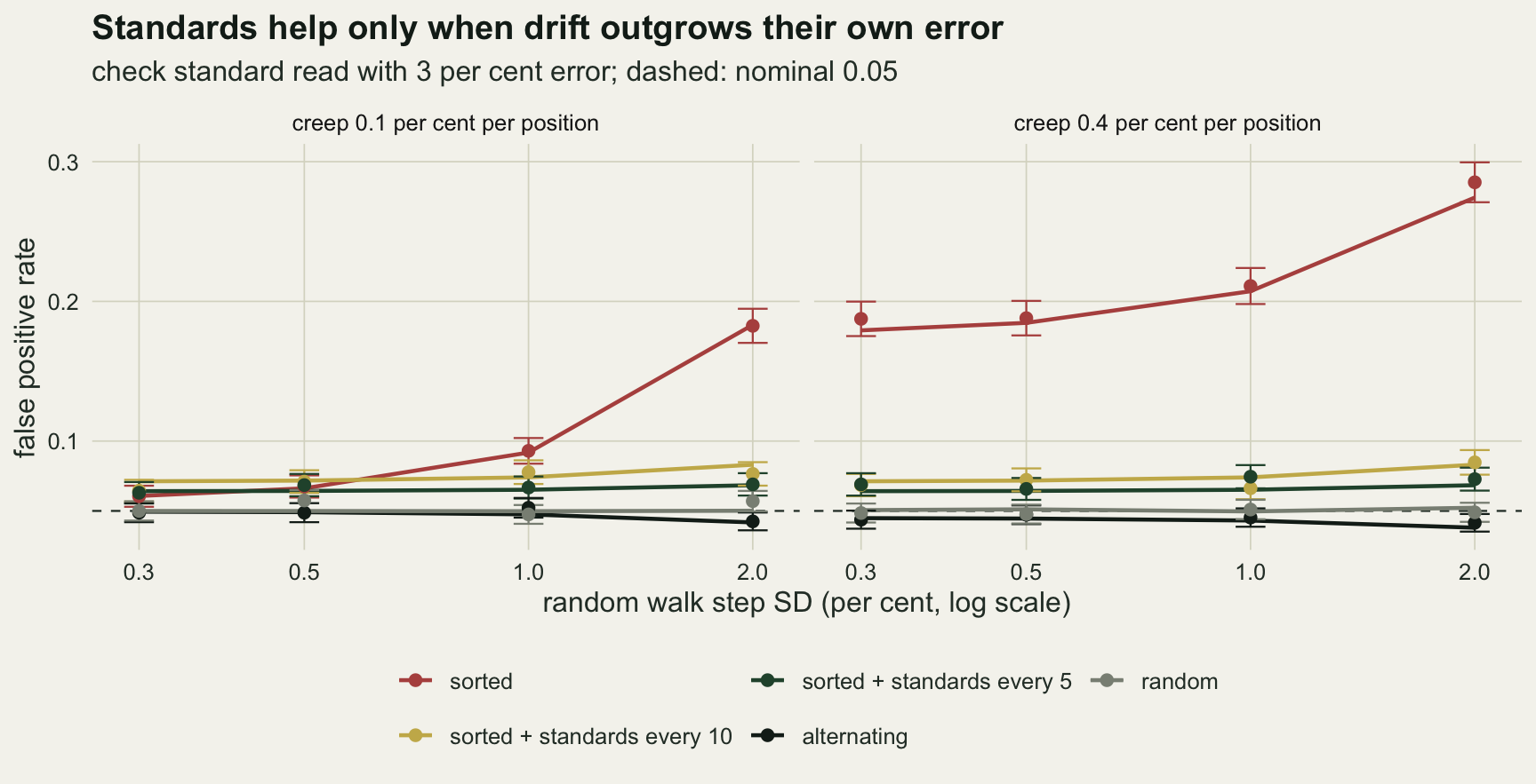

Figure 3: False positive rate against the size of the random walk step, for two creep rates. Points are simulations with two Monte Carlo standard errors; lines are the covariance calculation.

Power, and run position as a smooth

Once the order is alternating or random the confounding of a sorted run is gone, apart from the one-position lag of an alternating sheet taken up below, and the remaining question is whether the standards buy precision. A random walk adds variance to every reading, and interpolation removes part of it, while the standard’s own error adds some back. The next chunk measures power at a ten per cent effect across the walk sizes for both orders, with and without standards every five samples, over 20000 runs per cell because the differences to be seen are small.

A statistician’s alternative in a randomised run is to leave out the standards and estimate the drift from the samples themselves, with run position as a smooth term next to treatment. A penalised regression spline in mgcv does that, and because treatment is randomised with respect to position, the smooth has no systematic reason to absorb the effect. Fitting a model to each run is slow compared with the matrix t test, so that arm uses 1000 runs per setting, at the main drift.

n_pow <- 20000
set.seed(3105)
pow_designs <- data.frame(order = c("alternating", "alternating", "random", "random"),
                          k_std = c(0, 5, 0, 5), stringsAsFactors = FALSE)
power_res <- do.call(rbind, lapply(rw_grid, function(rw) {
  data.frame(pow_designs, rw = rw,
             power = mapply(function(o, k) sim_runs(o, k, lin_main, rw, eff = eff_10, n_rep = n_pow),
                            pow_designs$order, pow_designs$k_std))
}))
pow_of <- function(o, k, rw) power_res$power[power_res$order == o &
                                             power_res$k_std == k & power_res$rw == rw]
pow_diff_se <- sqrt(2) * mc_se(0.37, n_pow)
sim_changes <- c(pow_of("alternating", 5, 0.003) - pow_of("alternating", 0, 0.003),
                 pow_of("alternating", 5, 0.02) - pow_of("alternating", 0, 0.02),
                 pow_of("random", 5, 0.003) - pow_of("random", 0, 0.003),
                 pow_of("random", 5, 0.02) - pow_of("random", 0, 0.02))

lag_pred <- function(rw) {
  rbind(alt_none    = predict_rate(sheet_alt, 0, lin_main, rw, eff = eff_10),
        alt_nocreep = predict_rate(sheet_alt, 0, 0, rw, eff = eff_10),
        alt_std5    = predict_rate(sheet_alt, 5, lin_main, rw, eff = eff_10),
        rev_none    = predict_rate(!sheet_alt, 0, lin_main, rw, eff = eff_10),
        rev_std5    = predict_rate(!sheet_alt, 5, lin_main, rw, eff = eff_10))
}
lag_small <- lag_pred(0.003)
lag_large <- lag_pred(0.02)

n_gam <- 1000
gam_arm <- function(eff) {
  runs <- sim_runs("random", 0, lin_main, rw_main, eff = eff, n_rep = n_gam, keep = TRUE)
  pos  <- seq_len(n_smp)
  p_gam <- vapply(seq_len(n_gam), function(r) {
    fit_dat <- data.frame(y = runs$y[r, ], trt = as.numeric(runs$g[r, ]), pos = pos)
    fit <- gam(y ~ trt + s(pos, bs = "cr"), data = fit_dat, method = "REML")
    summary(fit)$p.table["trt", "Pr(>|t|)"]
  }, numeric(1))
  rej_gam <- p_gam < 0.05
  rej_t   <- abs(runs$t) > t_crit
  c(gam = mean(rej_gam), ttest = mean(rej_t),
    diff_se = sd(rej_gam - rej_t) / sqrt(n_gam))
}
gam_null  <- gam_arm(0)
gam_power <- gam_arm(eff_10)

With the smallest walk, 0.3 per cent a step, alternating runs reached a power of 0.3890 without standards and 0.3725 with them, a difference of 0.0164 against a standard error of 0.0048 for a difference. That difference is not a clean cost of the standards. The alternating sheet used here starts with a control, so every addition sample is read one position after its control, and the creep adds 0.004 to the difference in the direction of the effect. The calculator separates the parts. It predicts 0.3833 without standards, 0.3769 for the same sheet with the creep removed, and 0.3706 with standards every five, which take out a straight creep exactly. Of the predicted gap of 0.013, then, about half (0.0064) is the net effect of the creep, its push toward the effect less the spread it adds within each group, which the standards remove; the rest (0.0063) is their own reading error, less the little walk they take out. A sheet that starts with an addition plot turns the lag against the effect: 0.3319 without standards and 0.3706 with them, so there the standards gain power. The alternating power without standards in the grid of the earlier section carries the same lag. At the largest walk, 2 per cent a step, the simulated alternating runs gave 0.3520 without standards and 0.3635 with, and the calculator gives 0.3036 and 0.3642 for the sheet that starts with an addition plot. In randomised runs, where the lag averages out, the standards changed power by 0.0037 at the smallest walk, which is within noise, and added 0.0222 at the largest, because in a random order the drift inflates the within-group variance and interpolation takes some of it out. None of the simulated changes exceeds 0.0222, and the choice of which group a fixed alternating sheet starts with moves predicted power by up to 0.0514 across the two walks. The field variation is why the simulated changes stay small: a plot-to-plot standard deviation of 0.15 is far larger than what drift adds to an interspersed run, and no laboratory correction touches it.

The smooth of run position in a randomised run rejected a true null in 0.047 of 1000 runs, against 0.042 for the plain t test on the same runs, and its power at a ten per cent effect was 0.387 against 0.362. Because both tests saw the same runs, the relevant standard error is that of the paired difference: 0.0048 under the null and 0.0094 for power. The false positive rates differ by 1.0 paired standard errors, so the smooth kept its level as far as 1000 runs can tell, and the power gain is 2.7 paired standard errors. In a randomised run, estimating the drift from the samples themselves did a little better than ignoring it, and it needed no standards; the randomised runs with standards every five in the previous chunk reached 0.3683 at the same drift, from different simulated runs.

power_res$standards <- ifelse(power_res$k_std == 0, "no standards", "standards every 5")
power_res$se <- mc_se(power_res$power, n_pow)
ggplot(power_res, aes(100 * rw, power, colour = standards, linetype = standards)) +
  geom_line(linewidth = 0.8) +
  geom_errorbar(aes(ymin = power - 2 * se, ymax = power + 2 * se),
                width = 0.04, linewidth = 0.4, linetype = "solid") +
  geom_point(size = 2.2) +
  facet_wrap(~ order) +
  scale_x_log10(breaks = 100 * rw_grid) +
  scale_colour_manual(values = c("no standards" = te_rust,
                                 "standards every 5" = te_forest), name = NULL) +
  scale_linetype_manual(values = c("no standards" = "solid",
                                   "standards every 5" = "dashed"), name = NULL) +
  labs(x = "random walk step SD (per cent, log scale)", y = "power",
       title = "Interspersed runs: standards change power very little",
       subtitle = "creep 0.4 per cent per position; field SD 0.15") +
  theme_datasheet() +
  theme(legend.position = "bottom")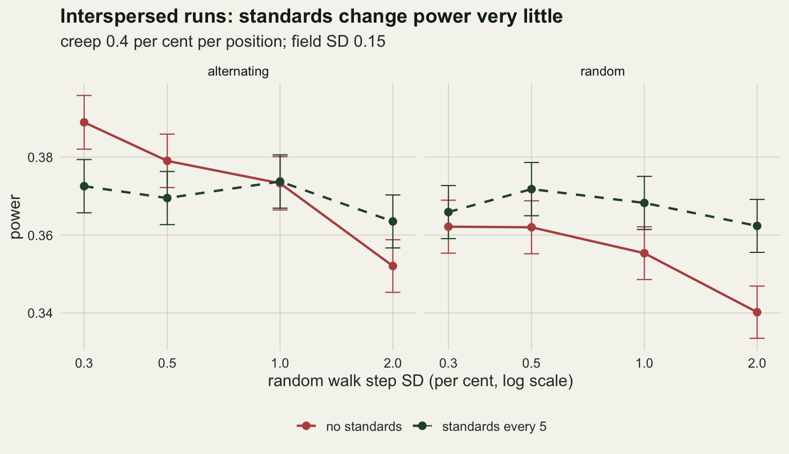

Figure 4: Power at a ten per cent true effect against random walk step size, for alternating runs (starting with a control plot) and randomised runs, with and without check standards every five samples. Bars are two Monte Carlo standard errors.

What to report

Report the run order, in words, next to the analytical method: sorted by treatment, alternating, randomised, or randomised within pairs. A methods section that says samples were analysed on an autoanalyser with check standards every ten samples has told a reader nothing about whether drift could have produced the treatment difference. Under the drift used here a sorted run rejected a true null in 0.202 of runs and a sorted run with standards every ten, read to 3 per cent, in 0.072.

Report the check standard results as numbers, not as a statement that they were within tolerance: the spacing, the reading error of the standard from its repeated readings, and the drift they show across the run. With those three the calculator above gives an approximate false positive rate for the sheet that was actually run, given the drift and standard error estimated from those readings. Keep the file with the order of the rack, because a reader who wants to check confounding needs the run position of every sample.

If a run has already gone through sorted, the data are not lost, but the standards will not rescue the test on their own. Two repairs are defensible, though neither was simulated here: treat the stretch between two standards as the unit that shares an error, or rerun a subset of samples in interspersed order to estimate the drift directly. Either way, the report says which was done.

Honest limits

The drift is a straight creep plus a Gaussian random walk on the log scale, the same for every sample. Real analysers also drift in steps, when a reagent bottle is changed or a tube is replaced, and some drift depends on concentration, so a standard near the bottom of the range does not correct a sample near the top. A single-level standard cannot follow a change in slope; laboratories that bracket the samples with low and high standards correct gain and offset separately, and that design was not simulated.

The drift magnitudes are assumptions, not measurements from any instrument. A creep of 0.4 per cent per position over a run of 37 readings, samples and standards together, is a 15 per cent change across an afternoon, which is meant as a badly behaved run rather than a typical one, and the sweep includes smaller values for that reason. Whether 1 or 2 per cent random steps per position are realistic depends on the instrument and the analyte, and a laboratory can answer it for its own instrument from the check standards it already reads. The zero-drift result does not depend on the drift at all, only on how precisely a standard is read relative to the field variation.

The field standard deviation of 0.15 decides much of the picture. With homogenised material, such as repeated analyses of one extract or laboratory incubations of a single soil, the between-sample variation can be a few per cent, and then both the drift and the standards’ shared error are large against it. The calculator handles that case by changing one constant, but the numbers in this post would all change.

Correction here is linear interpolation between neighbouring standards. Dunn and colleagues fit a smoother through all quality control readings of a run, which shares each reading’s error more widely and more thinly; that should shrink the shared error in a sorted run but cannot remove it, and it was not measured. The smooth of run position used a cubic regression basis with the default basis dimension and REML smoothing; a different basis dimension or smoothing criterion could change its rates slightly.

Only one analyte, one run and thirty samples were simulated. Large studies spread over several runs add a run effect, which is a batch in Leek’s sense and needs the same treatment: plots from every treatment in every run. Carryover between consecutive samples was not simulated either; it is systematic in an alternating sheet, where every addition sample follows a control, which is a second reason to randomise within pairs rather than alternate.

References

Box GEP, Hunter JS, Hunter WG 2005 Statistics for Experimenters: Design, Innovation, and Discovery, 2nd edition (ISBN 978-0-471-71813-0)

Dunn WB, Broadhurst D, Begley P, Zelena E, Francis-McIntyre S, Anderson N, Brown M, Knowles JD, Halsall A, Haselden JN, Nicholls AW, Wilson ID, Kell DB, Goodacre R 2011 Nature Protocols 6(7):1060-1083 (10.1038/nprot.2011.335)

Hurlbert SH 1984 Ecological Monographs 54(2):187-211 (10.2307/1942661)

Leek JT, Scharpf RB, Bravo HC, Simcha D, Langmead B, Johnson WE, Geman D, Baggerly K, Irizarry RA 2010 Nature Reviews Genetics 11(10):733-739 (10.1038/nrg2825)

Related tutorials

• Depth sensor drift and the dive count
• Pseudoreplication and false positives in ecology
• Values below the detection limit in R
• Checking your data against the design