library(ggplot2)
library(patchwork)

te_paper  <- "#f5f4ee"
te_ink    <- "#16241d"
te_body   <- "#2c3a31"
te_forest <- "#275139"
te_rust   <- "#b5534e"
te_gold   <- "#c9b458"
te_line   <- "#dad9ca"

theme_datasheet <- function() {
  theme_minimal(base_size = 12) +
    theme(plot.background  = element_rect(fill = te_paper, colour = NA),
          panel.background = element_rect(fill = te_paper, colour = NA),
          panel.grid.major = element_line(colour = te_line, linewidth = 0.3),
          panel.grid.minor = element_blank(),
          text             = element_text(colour = te_body),
          plot.title       = element_text(colour = te_ink, face = "bold"),
          plot.subtitle    = element_text(colour = te_body),
          axis.text        = element_text(colour = te_body))
}Depth sensor drift and the dive count
R
biologging
diving behaviour
measurement error
simulation
ecology tutorial
A slowly drifting pressure sensor zero changes the dive count of an unchanged animal. Simulating a dive record in R, predicting the loss, correcting the zero.
A fur seal carries a time-depth recorder glued to the fur between its shoulders for ten days. The tag writes one depth reading every five seconds for the whole deployment. Nobody reads those rows. They go through a dive detector, which marks every stretch of the record deeper than some threshold as a dive, and the analysis starts from the table that comes out: one row per dive, with a start time, a duration and a maximum depth. The number of dives per day, the mean maximum depth and the share of time spent submerged are the quantities that end up in the paper, and all of them are counted from a depth of zero.
That zero is not fixed. A pressure transducer reports depth as the difference between the pressure it measures and the pressure it believes corresponds to the surface, and the belief wanders: with temperature, with the age of the sensor, with the atmosphere above the sea. The wander is usually small, slow and smooth, a few tenths of a metre over days. It is invisible inside any single dive, because a dive to thirty metres that reads as twenty nine and a half is still a dive to about thirty metres. It is not invisible to a threshold.
Thresholds that decide a derived annual number are already covered here. Night-time flux and the u-star threshold estimates the friction velocity below which a night-time flux is thrown away and prices that choice in the annual carbon budget, and Check 1 of checking an annual flux budget bootstraps the same threshold through the whole pipeline. In both, the calibration of the instrument is taken as right and the uncertain object is the threshold. This post turns that around. The dive threshold is fixed at a sensible value and never changes; what moves is the instrument’s zero, slowly, underneath it. The site has named this kind of error before without modelling it: the honest limits of NDVI time series from a raster stack list among the things that simulation left out that “there is no sensor drift, so no slow change in calibration that a long series would read as a trend in greenness”. It is also a different animal from the drift in reporting rates and effort drift, where the recording effort of observers changes and the instrument is a person; here the observer is a transducer and the effort is constant.
The questions are what a linear zero drift does to the dive table of an animal whose behaviour does not change at all, whether the damage can be predicted before anyone has corrected anything, and how well the standard correction, zero offset correction from the readings taken at the surface, puts it back.
A ten day record from a diving predator
dt_s     <- 5      # seconds between depth samples
n_days   <- 10     # deployment length, days
thr_m    <- 3      # dive threshold, metres
min_n    <- 2      # a dive needs at least two consecutive samples below the threshold
noise_sd <- 0.15   # sensor noise, metres
v_speed  <- 1.2    # descent and ascent rate, metres per second
drift_md <- 0.4    # size of the zero offset drift, metres per day
day_s    <- 86400

sim_animal <- function(n_days, p_shallow, med_shallow = 4, med_deep = 30) {
  n_try <- ceiling(n_days * day_s / 60)
  deep  <- runif(n_try) > p_shallow
  maxd  <- ifelse(deep, rlnorm(n_try, log(med_deep), 0.4),
                  rlnorm(n_try, log(med_shallow), 0.5))
  bott  <- ifelse(deep, runif(n_try, 20, 60), runif(n_try, 5, 20))
  trav  <- maxd / v_speed
  surf  <- rgamma(n_try, shape = 2, scale = 45) + 0.5 * trav
  t_on  <- cumsum(c(0, (surf + 2 * trav + bott)[-n_try])) + surf
  keep  <- t_on + 2 * trav + bott < n_days * day_s
  maxd <- maxd[keep]; bott <- bott[keep]; trav <- trav[keep]; t_on <- t_on[keep]
  n_dv <- length(t_on)
  bdep <- maxd * runif(n_dv, 0.85, 1)
  first_max <- runif(n_dv) < 0.5
  knot_t <- as.vector(rbind(t_on, t_on + trav, t_on + trav + bott,
                            t_on + 2 * trav + bott))
  knot_d <- as.vector(rbind(0, ifelse(first_max, maxd, bdep),
                            ifelse(first_max, bdep, maxd), 0))
  time_s <- seq(0, n_days * day_s - dt_s, by = dt_s)
  depth  <- approx(c(0, knot_t, n_days * day_s), c(0, knot_d, 0), xout = time_s)$y
  list(time_s = time_s, depth = depth, n_dv = n_dv, maxd = maxd)
}
detect_dives <- function(time_s, depth, thr = thr_m) {
runs <- rle(depth > thr)
last <- cumsum(runs$lengths); first <- last - runs$lengths + 1
keep <- runs$values & runs$lengths >= min_n
first <- first[keep]; last <- last[keep]; len <- last - first + 1
dive_id <- rep.int(seq_along(first), len); idx <- sequence(len, first)
d_in <- depth[idx]
pair <- pmin(d_in, c(d_in[-1], -Inf)) # depth held for two samples
pair[c(diff(dive_id) != 0, TRUE)] <- -Inf
data.frame(start_s = time_s[first], dur_s = len * dt_s,
maxd = as.vector(tapply(d_in, dive_id, max)),
pairmax = as.vector(tapply(pair, dive_id, max)))
}
day_of <- function(s) floor(s / day_s) + 1
set.seed(4107)
seal <- sim_animal(n_days, p_shallow = 0.6)
dv_true <- detect_dives(seal$time_s, seal$depth)
rec_ref <- seal$depth + rnorm(length(seal$time_s), 0, noise_sd)
dv_ref <- detect_dives(seal$time_s, rec_ref)
n_below <- sum(seal$maxd <= thr_m)
n_gen <- seal$n_dv; n_true <- nrow(dv_true); n_ref <- nrow(dv_ref)
p_surface <- mean(seal$depth == 0)
share_near <- mean(dv_ref$maxd <= thr_m + drift_md * n_days)
budget <- function(dv, rec) c(n = nrow(dv), mean_max = mean(dv$maxd),
p_below = mean(rec > thr_m))
b_true <- budget(dv_true, seal$depth); b_ref <- budget(dv_ref, rec_ref)The design constants were fixed before any count was looked at: a sample every 5 seconds for 10 days, a dive threshold of 3 metres, sensor noise with a standard deviation of 0.15 metres, and a dive defined as at least 2 consecutive samples deeper than the threshold. The animal mixes two kinds of dive. Shallow dives have a median maximum depth of four metres and the deeper dives a median of thirty, with shallow dives making up sixty per cent of attempts; each dive descends and ascends at 1.2 metres per second with a short bottom phase, and surface intervals are drawn from a gamma distribution plus a term that grows with the depth of the dive they lead into. That design puts many shallow dives close to the threshold on purpose, because a coastal forager that works the kelp edge between bouts of deeper diving does exactly that.
The generator produced 5924 dive attempts, and the detector finds 4700 dives in the noise free depth. Of the difference, 1003 attempts never reached the threshold at all, and the remaining 221 crossed it for fewer than two samples or ran into a neighbouring dive across a very short surface interval. With sensor noise added and no drift at all it finds 4675. The noise free and noisy dive tables agree closely on the mean maximum depth (19.19 and 19.31 metres) and on the share of the deployment spent deeper than the threshold (29.3 and 29.3 per cent). The noisy record with no drift is the reference for everything below, because it is the best that this sensor could have done. The animal is at the surface for 65.8 per cent of the deployment, a number that will matter when the correction comes.
The same animal through a drifting sensor
offset_sh <- -drift_md * seal$time_s / day_s   # sensor creeps shallow
offset_dp <-  drift_md * seal$time_s / day_s   # sensor creeps deep
set.seed(4109)
noise_sh <- rnorm(length(seal$time_s), 0, noise_sd)
noise_dp <- rnorm(length(seal$time_s), 0, noise_sd)
rec_sh <- seal$depth + noise_sh + offset_sh
rec_dp <- seal$depth + noise_dp + offset_dp
drift_small <- 0.05   # metres per day, a mild drift on the same noise
rec_sh_small <- seal$depth + noise_sh - drift_small * seal$time_s / day_s
rec_dp_small <- seal$depth + noise_dp + drift_small * seal$time_s / day_s
chg_sh_small <- nrow(detect_dives(seal$time_s, rec_sh_small)) / nrow(dv_ref) - 1
chg_dp_small <- nrow(detect_dives(seal$time_s, rec_dp_small)) / nrow(dv_ref) - 1
dv_sh <- detect_dives(seal$time_s, rec_sh)
dv_dp <- detect_dives(seal$time_s, rec_dp)
b_sh <- budget(dv_sh, rec_sh); b_dp <- budget(dv_dp, rec_dp)
chg_sh <- b_sh["n"] / b_ref["n"] - 1; chg_dp <- b_dp["n"] / b_ref["n"] - 1
day_n <- function(dv) tabulate(day_of(dv$start_s), n_days)
daily <- data.frame(day = rep(seq_len(n_days), 3),
                    record = factor(rep(c("no drift", "creeping shallow", "creeping deep"),
                                        each = n_days),
                                    levels = c("no drift", "creeping shallow", "creeping deep")),
                    dives = c(day_n(dv_ref), day_n(dv_sh), day_n(dv_dp)))
d_ref <- day_n(dv_ref); d_sh <- day_n(dv_sh); d_dp <- day_n(dv_dp)
loss_d1 <- 1 - d_sh[1] / d_ref[1]; loss_d10 <- 1 - d_sh[n_days] / d_ref[n_days]
day_cross <- thr_m / drift_md
big_dp <- which.max(d_dp); longest_dp <- max(dv_dp$dur_s) / 3600
n_long_dp <- sum(dv_dp$dur_s > 3600)
The drifted records use the same animal and fresh sensor noise, with a zero offset that changes by 0.4 metres per day from zero at deployment. The sign needs defining, because the two directions do different things. A sensor creeping shallow reads every depth too shallow by the offset, so at the end of the deployment the surface reads as -4.0 metres. A sensor creeping deep reads every depth too deep, and the surface ends up at +4.0 metres.
That rate is deliberately severe. It takes the zero 4 metres from true in ten days, far beyond the few tenths of a metre described above, so that both ways of failing show up inside one deployment. For scale, the same animal and the same noise through a drift of 0.05 metres per day, which ends 0.5 metres off, changes the dive count by -4.6 per cent creeping shallow and by +4.4 per cent creeping deep. The sweep further down fills in the rates between.
Creeping shallow, the detector finds 3535 dives instead of 4675, a change of -24.4 per cent in an animal that did exactly the same thing. The dives that vanish are the shallow ones, so the survivors are deeper on average and the mean maximum depth moves from 19.31 to 22.31 metres, a shift of +3.00 metres, even though every recorded depth was reported too shallow. The two errors pull in opposite directions and the selection wins. The share of time below the threshold falls from 29.3 to 25.9 per cent.
Creeping deep, the dive count goes up, to 5348 (+14.4 per cent), and the mean maximum depth falls to 16.19 metres, because surface noise and the shallowest excursions start to cross the threshold. The share of time below the threshold becomes 49.1 per cent. Neither whole deployment number describes what happened, which the daily counts make plain.
win_min <- 40
ex_start <- c(1, 10)
ex <- do.call(rbind, lapply(ex_start, function(dd) {
  i0 <- ((dd - 1) * day_s + 12 * 3600) / dt_s + 1
  ii <- i0:(i0 + win_min * 60 / dt_s)
  data.frame(minute = (seal$time_s[ii] - seal$time_s[i0]) / 60,
             true = seal$depth[ii], recorded = rec_sh[ii],
             panel = sprintf("day %d, offset %+.1f m", dd, offset_sh[i0]))
}))
ggplot(ex, aes(minute)) +
  geom_hline(yintercept = thr_m, colour = te_rust, linetype = "dashed", linewidth = 0.6) +
  geom_line(aes(y = true), colour = te_gold, linewidth = 1.5) +
  geom_line(aes(y = recorded), colour = te_forest, linewidth = 0.5) +
  scale_y_reverse(breaks = seq(-5, 15, 5)) +
  coord_cartesian(ylim = c(15, -5)) +
  facet_wrap(~ panel, ncol = 1) +
  labs(x = "minutes from noon", y = "depth (m)",
       title = "The same animal, ten days apart",
       subtitle = "gold: true depth, green: recorded, dashed: 3 m threshold; axis cut at 15 m") +
  theme_datasheet() +
  theme(strip.text = element_text(colour = te_ink, face = "bold", hjust = 0))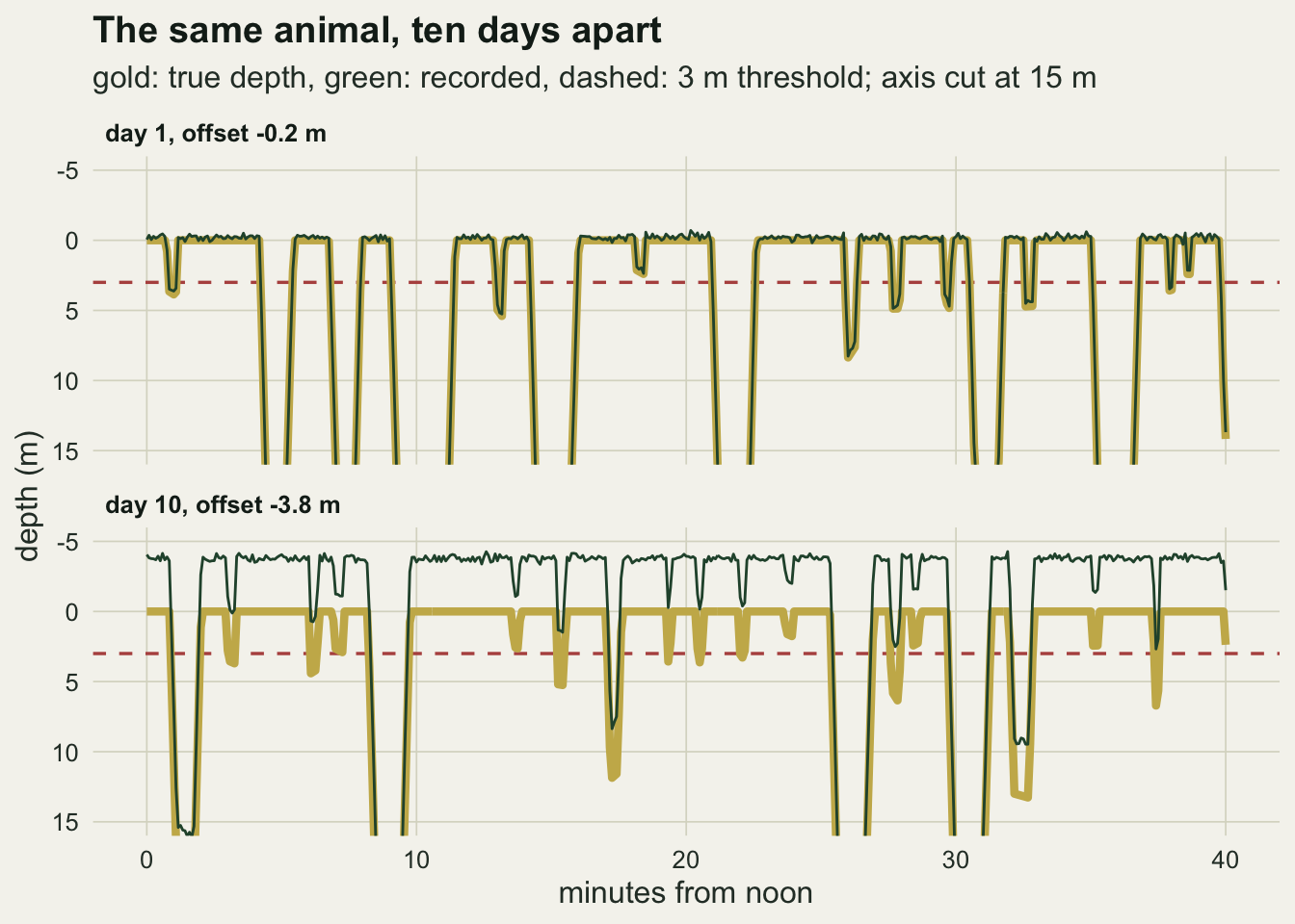
y_cap <- 800
ggplot(daily, aes(day, pmin(dives, y_cap), colour = record)) +
  geom_line(linewidth = 0.9) + geom_point(size = 2.2) +
  annotate("text", x = big_dp, y = y_cap, vjust = -0.6, colour = te_rust,
           label = sprintf("%d (off scale)", d_dp[big_dp])) +
  scale_colour_manual(values = c(te_ink, te_gold, te_rust), name = NULL) +
  scale_x_continuous(breaks = seq_len(n_days)) +
  coord_cartesian(ylim = c(0, y_cap * 1.08)) +
  labs(x = "day of deployment", y = "dives detected",
       title = "A linear drift, two very different failures",
       subtitle = "one animal, three records of it") +
  theme_datasheet() + theme(legend.position = "bottom")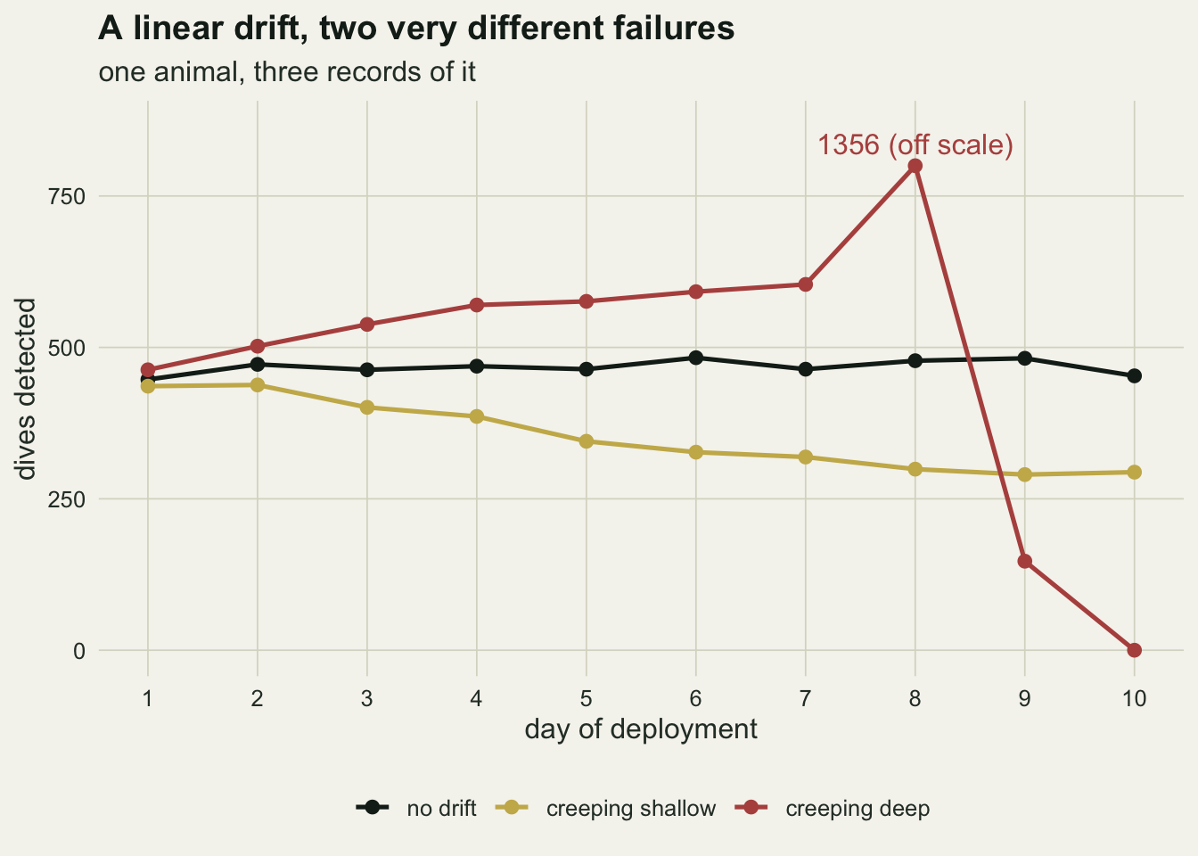
The excerpt shows the mechanism at the scale of single dives. On the first day the recorded and true profiles lie on top of each other. On the last day the recorded trace is lifted by nearly four metres everywhere, the surface reads as a negative depth, and every shallow dive that the true profile carries past the dashed line in this window no longer reaches it in the record. The deeper dives run off the bottom of the panel on both days and are detected either way.
Creeping shallow, the first day loses 2.5 per cent of its dives against the reference and the last day loses 35.1 per cent. The drift is a straight line; the daily loss is not, and it flattens as the days go on. Creeping deep, the count rises for a week. As the offset approaches the threshold, which it reaches at day 7.5, the surface readings straddle it, and sensor noise chops every surface interval into a burst of tiny dives: 1356 on day 8. Once the offset is a couple of noise standard deviations past the threshold, no surface reading falls back above it, and the rest of the record merges into 3 dives longer than an hour, the longest lasting 33.3 hours. A seal that dived as usual for ten days appears to make 147 dives on day 9 against 482 in the reference, and 0 on day 10.
The loss is the depth distribution read at a moving threshold
rates <- c(0.05, 0.1, 0.2, 0.3, 0.4, 0.6, 0.8)   # metres per day, shallow creep
set.seed(4108)
diver   <- sim_animal(n_days, p_shallow = 0.2)
rec_ref_b <- diver$depth + rnorm(length(diver$time_s), 0, noise_sd)
dv_ref_b  <- detect_dives(diver$time_s, rec_ref_b)
pred_loss <- function(dv, rate, col) 1 - mean(dv[[col]] - rate * dv$start_s / day_s > thr_m)
set.seed(4110)
sweep_one <- function(an, dvr, lab) do.call(rbind, lapply(rates, function(r) {
  rec <- an$depth + rnorm(length(an$time_s), 0, noise_sd) - r * an$time_s / day_s
  data.frame(animal = lab, rate = r, end_offset = r * n_days,
             loss_meas = 1 - nrow(detect_dives(an$time_s, rec)) / nrow(dvr),
             loss_max  = pred_loss(dvr, r, "maxd"),
             loss_pair = pred_loss(dvr, r, "pairmax"))
}))
lab_mix <- "mixed forager"; lab_deep <- "deep forager"
sw <- rbind(sweep_one(seal, dv_ref, lab_mix), sweep_one(diver, dv_ref_b, lab_deep))
sw$animal <- factor(sw$animal, levels = c(lab_mix, lab_deep))
gap_pair <- max(abs(sw$loss_meas - sw$loss_pair))
gap_max  <- max(abs(sw$loss_meas - sw$loss_max))
at_r <- function(lab, r, col) sw[[col]][sw$animal == lab & sw$rate == r]
near_b <- mean(dv_ref_b$maxd <= thr_m + drift_md * n_days)
p_surface_b <- mean(diver$depth == 0)
first_step <- at_r(lab_mix, 0.1, "loss_meas") / (0.1 * n_days)
last_step  <- (at_r(lab_mix, 0.8, "loss_meas") - at_r(lab_mix, 0.6, "loss_meas")) / (0.2 * n_days)
loss_big <- max(sw$loss_meas)
se_loss  <- sqrt(loss_big * (1 - loss_big) / nrow(dv_ref))   # binomial error of one loss
The sweep runs a sensor creeping shallow at 7 rates, from 0.05 to 0.8 metres per day, through two animals: the mixed forager above, and a deep forager that makes shallow dives on only twenty per cent of attempts. Each drifted record gets its own noise.
The prediction needs no drifted record at all. A drift creeping shallow by an offset at time t removes a dive exactly when the dive would no longer have held the threshold plus that offset, so the loss can be read from the reference dive table by moving the threshold along with the drift. The first version of the rule uses the maximum depth of each dive, since that is the column everyone has. The second uses the greatest depth the dive held for two consecutive samples, which is what the dive definition actually requires.
Measured and predicted losses for both animals are in the figure below. The rule based on the depth held for two samples misses the measured loss by at most 0.5 percentage points across all 14 drifted records. The rule based on maximum depth underpredicts by up to 3.4 points: a dive whose single deepest sample clears the moved threshold can still be lost because the sample before or after it does not. Each rate is one drifted record with its own noise. A binomial standard error for a loss of 35.3 per cent on 4675 dives is 0.7 percentage points, so the two sample rule agrees with the measurement to within the error of a single record, and the gap of the maximum depth rule is larger than that error.
At 0.4 metres per day the mixed forager loses 24.4 per cent of its dives and the deep forager 6.8 per cent. The drift is identical; the difference is how many dives each animal makes to depths just past the threshold. In the reference tables 38.6 per cent of the mixed forager’s dives have a maximum depth between 3 and 7 metres, against 11.1 per cent for the deep forager. The measured loss is smaller than those shares because the offset only reaches its full size on the last day.
The curvature is the shape of the depth distribution. For the mixed forager the first metre of shallow offset at the end of the deployment costs 8.3 percentage points per metre, and the step from six to eight metres of offset costs 2.2 points per metre. Maximum depths are dense just deeper than the threshold and sparse further down, so the first metre of offset does 3.8 times the harm of a metre added beyond six.
sw_long <- rbind(data.frame(sw[, c("animal", "end_offset")], rule = "maximum depth",
                            loss = sw$loss_max),
                 data.frame(sw[, c("animal", "end_offset")], rule = "depth held two samples",
                            loss = sw$loss_pair))
ggplot(sw, aes(end_offset)) +
  geom_line(data = sw_long, aes(y = 100 * loss, colour = animal, linetype = rule),
            linewidth = 0.8) +
  geom_point(aes(y = 100 * loss_meas, colour = animal), size = 2.4) +
  scale_colour_manual(values = c(te_forest, te_gold), name = NULL) +
  scale_linetype_manual(values = c("solid", "dashed"), name = "predicted from") +
  guides(colour = guide_legend(order = 1), linetype = guide_legend(order = 2)) +
  labs(x = "size of the shallow offset at the end of the deployment (m)",
       y = "dives lost (per cent)",
       title = "Same drift, different animals, different losses",
       subtitle = "points: measured on a drifted record, lines: predicted from the clean dive list") +
  theme_datasheet() + theme(legend.position = "bottom", legend.box = "vertical")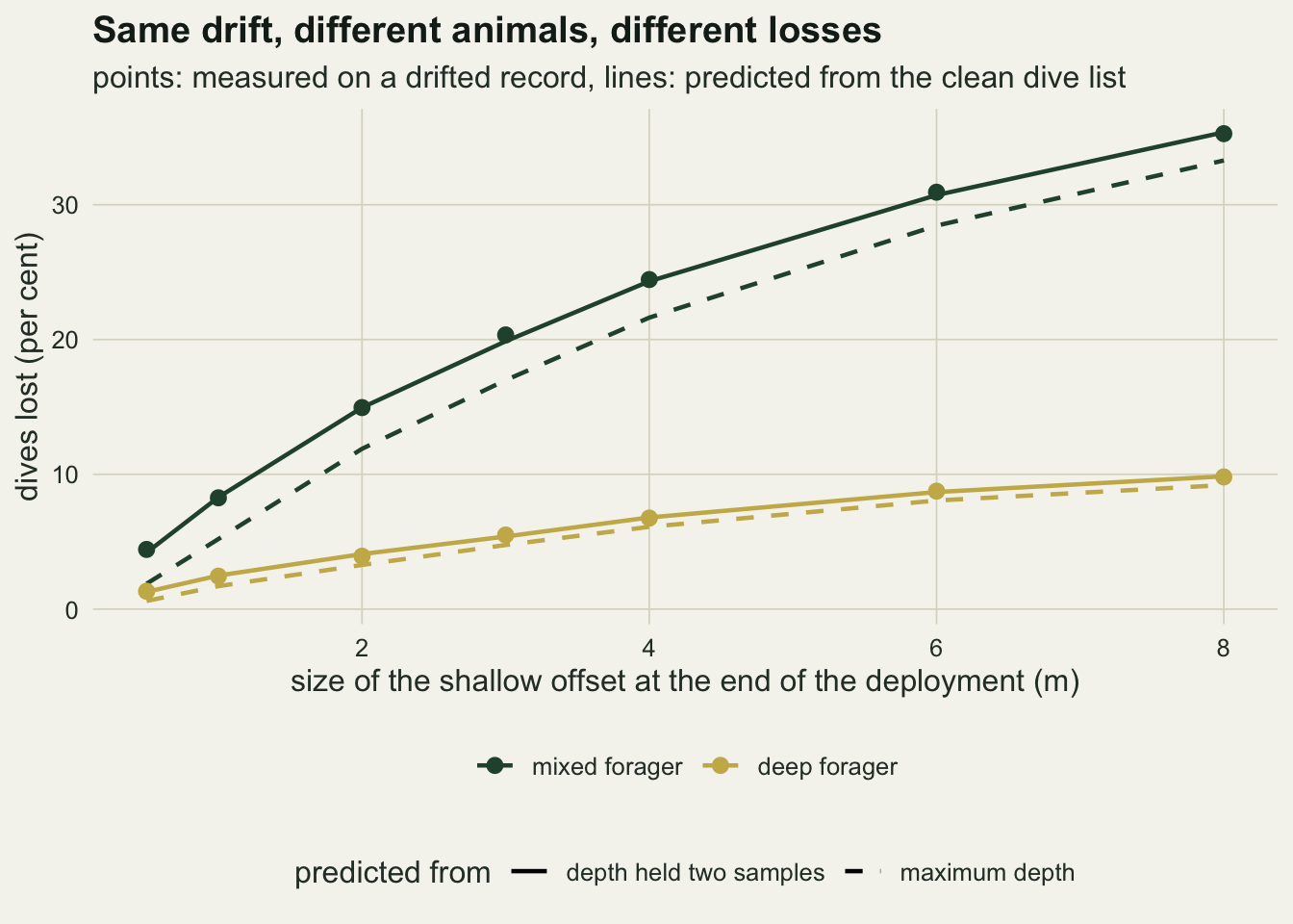
Zero offset correction from the surface
The correction exploits the one depth an air breathing diver keeps returning to. Whatever the sensor reads while the animal floats between dives is the zero offset plus noise, so the offset can be estimated from the surface readings and subtracted. Luque and Fried 2011 built this into the diveMove package as a procedure that smooths and filters the record recursively with moving quantiles, and evaluated it by corrupting a clean record from an Antarctic fur seal and comparing the corrected record with the original. The version below is a simplified two pass relative of that idea, written in base R so every step is visible. It is not the diveMove filter. In each hour it takes a low quantile of the readings as a rough surface level, keeps the readings within half a metre of it, takes their median as the offset for that hour, and interpolates linearly between hours.
zoc_offset <- function(time_s, rec, win_h = 1, band = 0.5) {
  hr <- floor(time_s / (win_h * 3600))
  coarse  <- tapply(rec, hr, quantile, probs = 0.05)[as.character(hr)]
  at_surf <- abs(rec - coarse) < band
  med <- tapply(rec[at_surf], hr[at_surf], median)
  mid <- (as.numeric(names(med)) + 0.5) * win_h * 3600
  approx(mid, med, xout = time_s, rule = 2)$y
}
est_sh <- zoc_offset(seal$time_s, rec_sh); est_dp <- zoc_offset(seal$time_s, rec_dp)
cor_sh <- rec_sh - est_sh; cor_dp <- rec_dp - est_dp
dv_csh <- detect_dives(seal$time_s, cor_sh); dv_cdp <- detect_dives(seal$time_s, cor_dp)
b_csh <- budget(dv_csh, cor_sh); b_cdp <- budget(dv_cdp, cor_dp)
err_sh <- est_sh - offset_sh; err_dp <- est_dp - offset_dp
err_max <- max(abs(c(err_sh, err_dp))); err_mean <- mean(c(err_sh, err_dp))
set.seed(4111)
rec_b_sh <- diver$depth + rnorm(length(diver$time_s), 0, noise_sd) -
            drift_md * diver$time_s / day_s
dv_b_sh  <- detect_dives(diver$time_s, rec_b_sh)
dv_b_cor <- detect_dives(diver$time_s, rec_b_sh - zoc_offset(diver$time_s, rec_b_sh))
chg_b_raw <- nrow(dv_b_sh) / nrow(dv_ref_b) - 1
chg_b_cor <- nrow(dv_b_cor) / nrow(dv_ref_b) - 1
sens_half <- mean(dv_csh$pairmax <= thr_m + 0.5)   # dives lost if the zero were half a metre wrong
hr_i <- seq(1, length(seal$time_s), by = 60)
err_df <- data.frame(day = rep(seal$time_s[hr_i] / day_s, 2),
err_cm = 100 * c(err_sh[hr_i], err_dp[hr_i]),
record = rep(c("creeping shallow", "creeping deep"), each = length(hr_i)))
p_err <- ggplot(err_df, aes(day, err_cm, colour = record)) +
geom_hline(yintercept = 0, colour = te_body, linewidth = 0.4) +
geom_line(linewidth = 0.4) +
scale_colour_manual(values = c(te_rust, te_gold), name = NULL) +
scale_x_continuous(breaks = seq(0, n_days, 2)) +
labs(x = "day of deployment", y = "offset error (cm)",
title = "Estimated minus true offset") +
theme_datasheet() + theme(legend.position = "bottom")
daily_c <- data.frame(day = rep(seq_len(n_days), 3),
record = factor(rep(c("no drift", "shallow, corrected", "deep, corrected"),
each = n_days),
levels = c("no drift", "shallow, corrected", "deep, corrected")),
dives = c(d_ref, day_n(dv_csh), day_n(dv_cdp)))
p_cnt <- ggplot(daily_c, aes(day, dives, colour = record)) +
geom_line(linewidth = 0.9) + geom_point(size = 1.8) +
scale_colour_manual(values = c(te_ink, te_gold, te_rust), name = NULL) +
scale_x_continuous(breaks = seq(2, n_days, 2)) +
coord_cartesian(ylim = c(0, 800)) +
guides(colour = guide_legend(nrow = 2)) +
labs(x = "day of deployment", y = "dives detected", title = "Dives after correction") +
theme_datasheet() + theme(legend.position = "bottom")
p_err + p_cnt + plot_annotation(theme = theme_datasheet())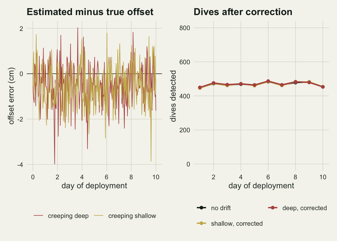
The estimated offset is never more than 4.0 centimetres from the true one in either direction of drift, against a true offset that reaches 400 centimetres, and its mean error is -0.5 centimetres. After subtraction the detector finds 4674 dives in the record that crept shallow and 4694 in the one that crept deep, against 4675 with no drift. Mean maximum depths come back as 19.32 and 19.25 metres against 19.31. The collapse after day 7.5 is gone as well, because the correction never lets the surface drift towards the threshold. For the deep forager, which spends 55.7 per cent of the deployment at the surface, the same drift on a fresh noise draw changes the count by -7.0 per cent uncorrected (the sweep record at this rate lost 6.8 per cent) and by +0.1 per cent corrected.
This correction works so well here because the simulated animal gives it everything it needs: long, frequent, flat surface intervals, and a drift that changes by 1.7 centimetres within an hour. The honest limits below say where that stops being true.
What to report
Report the zero offset correction as part of the method, not as preprocessing: the window, the quantile, the band around the surface, and the range the estimated offset covered over the deployment. A reader who sees that the offset moved by several metres knows the uncorrected dive table would have been different, and in which direction.
Report the dive threshold together with the minimum duration, because the dive definition is both. The sweep above shows that a loss predicted from maximum depth alone falls short of the measured loss by up to 3.4 percentage points, and all but 0.5 points of that gap is the duration rule.
Report how sensitive the count is to the zero. The corrected dive table already contains the answer: in the mixed forager’s corrected record, 7.8 per cent of dives held the threshold by less than half a metre for two samples, so an undetected offset of half a metre creeping shallow would remove about that share. One line in the methods, computed from data the study already has, tells a reader whether a residual error in the zero could matter for this animal.
Compare dive counts across individuals or species only when both the threshold and the depth distribution near it are stated. The same drift cost the two simulated animals very different shares of their dives, so a difference in dive rate between a shallow and a deep forager can be partly a difference in how many dives each makes to depths just past the threshold.
Honest limits
The drift here is a straight line in time. Real zero offsets move with water temperature as well as with time, so a tag that alternates between warm surface water and cold water at depth can carry an offset that changes within a single dive, and some sensors jump in steps after a pressure shock. An hourly surface median cannot follow anything faster than an hour, and a within dive temperature effect is invisible to any surface based correction.
Only the offset drifts. Pressure transducers also have a gain error, a proportional error that makes deep readings wrong by more than shallow ones. A gain error hardly touches the dive count at a three metre threshold but moves maximum depths of the deepest dives directly, and surface readings carry no information about it; it needs a calibration against known depths.
The simulated forager surfaces often and floats still. Animals that rest or sleep at depth, animals that spend long bouts without a proper surface interval, and animals whose surface time is shorter than the sampling interval all break the assumption that the lowest readings in an hour are the surface. The low quantile will then find the shallow end of the dive bouts instead, and the correction will subtract part of the behaviour. The diveMove procedure leaves its windows and quantiles to the user, and the settings have to be chosen for the species.
Dive profiles are piecewise straight lines with smooth bottoms, the sea is flat, and the sensor noise is independent from sample to sample with no rounding to a resolution step. Wave motion at the surface widens the surface readings, a coarse depth resolution quantises them, and both make the surface median less precise than the few centimetres found here. The five second interval is also coarse for shallow dives; at one second the duration rule should remove fewer dives and narrow the gap between the two predictions, which was not tested here.
The prediction of the loss uses the dive table of the undrifted record. In practice that table does not exist; the nearest thing is the corrected table, so what the rule can really give is the sensitivity of the count to a residual error in the zero, as in the half metre example above, not a reconstruction of damage that has already happened.
The design has one threshold, one noise level and two animals. Halsey and colleagues 2007 set out a quantified method for classifying seabird dives from depth records, and a classification of that kind is measured from the same zero. Studies of animals that go very much deeper, such as the northern bottlenose whales tagged by Hooker and Baird 1999, record dives deeper than a kilometre and need sensors with a full scale range larger still, where a small fraction of full scale is already metres of offset; the numbers above say nothing about those instruments directly, only about how an offset of a given size meets a threshold.
References
Luque SP, Fried R 2011 PLoS ONE 6(1):e15850 (10.1371/journal.pone.0015850)
Halsey LG, Bost CA, Handrich Y 2007 Polar Biology 30(8):991-1004 (10.1007/s00300-007-0257-3)
Hooker SK, Baird RW 1999 Proceedings of the Royal Society B 266(1420):671-676 (10.1098/rspb.1999.0688)