library(ggplot2)
library(patchwork)

te_paper  <- "#f5f4ee"
te_ink    <- "#16241d"
te_body   <- "#2c3a31"
te_forest <- "#275139"
te_rust   <- "#b5534e"
te_gold   <- "#c9b458"
te_line   <- "#dad9ca"

theme_datasheet <- function() {
  theme_minimal(base_size = 12) +
    theme(plot.background  = element_rect(fill = te_paper, colour = NA),
          panel.background = element_rect(fill = te_paper, colour = NA),
          panel.grid.major = element_line(colour = te_line, linewidth = 0.3),
          panel.grid.minor = element_blank(),
          text             = element_text(colour = te_body),
          plot.title       = element_text(colour = te_ink, face = "bold"),
          plot.subtitle    = element_text(colour = te_body),
          axis.text        = element_text(colour = te_body))
}Sap flow and the zero-flow baseline
R
ecophysiology
sap flow
measurement error
simulation
ecology tutorial
Thermal dissipation sap flow needs a zero-flow baseline. Simulating in R how night transpiration and probe noise bias tree water use under each baseline rule.
A beech stand on a slope has a thermal dissipation probe in every monitored stem. Each probe is a pair of needles in the sapwood: the upper one is heated with constant power, the lower one is not, and a logger writes the temperature difference between them every fifteen minutes for the whole season. When sap moves, it carries heat away from the heated needle and the difference shrinks; when sap stops, the difference climbs to its largest value. Granier 1985 turned that into a calibration. The ratio of the zero-flow difference minus the current difference to the current difference is raised to the power 1.231 and multiplied by a constant, and the result is a sap flux density. Summed over a month and scaled by sapwood area, it becomes the water use of the tree.
Everything in that calibration is anchored to one number the probe never reports directly: the temperature difference at zero flow. The usual answer is to take it from the night, when the stomata are shut and the stem should be still, as the largest difference recorded before dawn. Regalado and Ritter 2007 put the problem in two sentences: sap flow may continue during the night, so the predawn maximum can be lower than the true zero-flow value, and an error in that value is amplified by Granier’s formula, so a small undetected night flow produces a large daytime error. Oishi, Hawthorne and Oren 2016 wrote Baseliner, an interactive program for processing these records, because no set of algorithms reliably picks the baseline and a person ends up inspecting it by eye. Peters and colleagues 2018 quantified how processing choices move conifer water use and found that commonly applied methods mostly underestimate sap flux density.
The zero of an instrument has been corrected on this site before. Depth sensor drift and the dive count estimates a drifting pressure zero from the readings taken while a seal floats at the surface, and that works because an air breathing diver returns to its zero every few minutes. A tree has no such obligation. On a warm, dry, windy night the stem keeps moving water, and the zero-flow state may not occur for several nights in a row. Night-time flux and the u-star threshold also treats the night as a data problem, but for a flux tower, where calm nights are the unreliable ones; here calm nights are the only reliable ones. The second error in this post is the maximum of noisy values, which net primary production from repeated harvests meets as an inflated peak standing crop, and records as a test for trend meets as the running record of a series.
The post does three things. It shows that each error on its own, a steady night flow or noise in the readings, has a size that follows from arithmetic, and checks the simulation against that arithmetic rather than presenting it as a finding. It then lets night flow vary from night to night and compares baseline rules as the share of calm nights changes, which is where no formula is available. Finally it shows that the multi-night envelope trades one error for the other, and that averaging the predawn readings before taking any maximum removes most of the noise part.
A month of readings from one probe
The generating model has five parts, and all of its constants are fixed in the chunk below, before anything is run.
alpha_g <- 42.84; beta_g <- 1.231
n_day <- 30; step_h <- 0.25
hrs <- seq(0, n_day * 24 - step_h, by = step_h); n_t <- length(hrs)
hod <- hrs %% 24; day_id <- floor(hrs / 24) + 1
night_id <- floor((hrs + 6) / 24) + 1
is_pre <- hod < 6; is_late <- hod >= 4 & hod < 6
is_night <- hod >= 18 | hod < 6
shape_day <- ifelse(hod >= 6 & hod < 18, sin(pi * (hod - 6) / 12)^1.5, 0)
dtmax0 <- 10; u_peak <- 15; cv_day <- 0.3
wander_sd <- 0.1; wander_phi <- 0.8
vpd_mean <- 0.5; vpd_thr <- 0.1
n_tree <- 150
n_night <- n_day + 1
t_night <- (seq_len(n_day) - 1) * 24 + 3
lo_n <- pmin(pmax(findInterval(hrs, t_night), 1), n_day - 1)
w_n  <- pmin(pmax((hrs - t_night[lo_n]) / 24, 0), 1)

simulate_trees <- function(n_tree, fn, p_calm, noise_sd, wander = wander_sd,
                           cv = cv_day, vpd_const = FALSE) {
  demand <- matrix(u_peak * exp(rnorm(n_tree * n_day, -cv^2 / 2, cv)), n_tree)
  if (vpd_const) {
    vpd <- matrix(vpd_mean, n_tree, n_night)
  } else {
    vpd <- matrix(rexp(n_tree * n_night, 1 / vpd_mean), n_tree) *
           (runif(n_tree * n_night) > p_calm)
  }
  u_day   <- demand[, day_id, drop = FALSE] * rep(shape_day, each = n_tree)
  u_night <- fn * u_peak * vpd[, night_id, drop = FALSE] / vpd_mean *
             rep(is_night, each = n_tree)
  u_true <- pmax(u_day, u_night)
  wand <- matrix(0, n_tree, n_night)
  wand[, 1] <- rnorm(n_tree, 0, wander)
  for (k in 2:n_night) {
    wand[, k] <- wander_phi * wand[, k - 1] + sqrt(1 - wander_phi^2) * rnorm(n_tree, 0, wander)
  }
  dtmax_true <- dtmax0 + wand[, lo_n, drop = FALSE] * rep(1 - w_n, each = n_tree) +
                wand[, lo_n + 1, drop = FALSE] * rep(w_n, each = n_tree)
  k_true <- (u_true / alpha_g)^(1 / beta_g)
  dT <- dtmax_true / (1 + k_true) + matrix(rnorm(n_tree * n_t, 0, noise_sd), n_tree)
  list(u_true = u_true, dT = dT, dtmax_true = dtmax_true, vpd = vpd[, seq_len(n_day), drop = FALSE])
}
Daytime flux density follows a sine shape between 06:00 and 18:00 with a peak that varies from day to day (lognormal, coefficient of variation 0.3, median near 15 cm3 per cm2 per hour). Night flow runs from 18:00 to 06:00 at a level set by that night’s vapour pressure deficit: a calm night has a deficit of zero and no flow, any other night draws its deficit from an exponential distribution with mean 0.5 kPa, and the night flow is a fraction of the daytime peak scaled by the deficit over its mean. The true zero-flow difference wanders around 10 K as a daily autoregressive process (standard deviation 0.1 K, lag one correlation 0.8). The probe reading is the Granier relation run backwards plus Gaussian noise. The Granier constant is 118.99 millionths of a metre per second, which is 42.84 cm3 per cm2 per hour.
Every baseline rule below turns the readings into one zero-flow value per night, placed at 03:00 and interpolated linearly between nights. The daily predawn maximum takes the largest reading between 00:00 and 06:00. The predawn mean takes the average of the eight readings between 04:00 and 06:00. An envelope takes the largest nightly value in a centred window of several nights; that is a simplification of the automated baseline steps in processing tools such as Baseliner, not a reimplementation of any of them. The low deficit rule keeps only the predawn maxima of nights whose deficit was below 0.1 kPa and interpolates between those; a tree with fewer than two such nights falls back to the seven night envelope.
nightly <- function(dT, keep, fun) {
  per <- sum(keep) / n_day
  arr <- array(dT[, keep, drop = FALSE], c(nrow(dT), per, n_day))
  if (identical(fun, "mean")) return(rowMeans(aperm(arr, c(1, 3, 2)), dims = 2))
  out <- arr[, 1, , drop = TRUE]
  for (r in 2:per) out <- pmax(out, arr[, r, , drop = TRUE])
  out
}
by_day <- function(m) rowSums(aperm(array(m, c(nrow(m), 96, n_day)), c(1, 3, 2)), dims = 2)
run_max <- function(bm, wd) {
  h <- (wd - 1) / 2; out <- bm; idx <- seq_len(ncol(bm))
  if (h > 0) for (s in seq_len(h)) {
    out <- pmax(out, bm[, pmin(idx + s, ncol(bm)), drop = FALSE], bm[, pmax(idx - s, 1), drop = FALSE])
  }
  out
}
spread_night <- function(bm) bm[, lo_n, drop = FALSE] * rep(1 - w_n, each = nrow(bm)) +
                             bm[, lo_n + 1, drop = FALSE] * rep(w_n, each = nrow(bm))
flux_from <- function(base_t, dT) alpha_g * pmax((base_t - dT) / dT, 0)^beta_g
low_vpd_base <- function(pre_max, vpd, env7) {
  n_fall <- 0
  out <- t(vapply(seq_len(nrow(pre_max)), function(i) {
    ok <- vpd[i, ] < vpd_thr
    if (sum(ok) < 2) { n_fall <<- n_fall + 1; return(env7[i, ]) }
    approx(t_night[ok], pre_max[i, ok], xout = t_night, rule = 2)$y
  }, numeric(n_day)))
  attr(out, "n_fall") <- n_fall
  out
}
score_rules <- function(sim, windows = c(3, 7, 11), daily = FALSE) {
  dT <- sim$dT; use_true <- rowSums(sim$u_true)
  pre_max  <- nightly(dT, is_pre, "max")
  pre_mean <- nightly(dT, is_late, "mean")
  bases <- list(predawn_max = pre_max, predawn_mean = pre_mean)
  for (wd in windows) {
    bases[[paste0("env_max_", wd)]]  <- run_max(pre_max, wd)
    bases[[paste0("env_mean_", wd)]] <- run_max(pre_mean, wd)
  }
  if (7 %in% windows) {
    lv <- low_vpd_base(pre_max, sim$vpd, bases$env_max_7)
    bases$low_vpd <- lv
  }
  est <- lapply(bases, function(bm) flux_from(spread_night(bm), dT))
  est$true_base <- flux_from(sim$dtmax_true, dT)
  ratio <- sapply(est, function(e) rowSums(e) / use_true)
  out <- list(ratio = ratio, n_fall = if (7 %in% windows) attr(lv, "n_fall") else NA)
  if (daily) {
    day_true <- by_day(sim$u_true)
    out$daily <- lapply(est, function(e) by_day(e) / day_true)
  }
  out
}set.seed(3107)
fn_main <- 0.1; calm_main <- 0.25; sd_main <- 0.1
sim_main <- simulate_trees(n_tree, fn_main, calm_main, sd_main)
sc_main <- score_rules(sim_main, daily = TRUE)
show_h <- hrs < 10 * 24
tr <- 1
pre_max_1 <- nightly(sim_main$dT, is_pre, "max")
pre_mean_1 <- nightly(sim_main$dT, is_late, "mean")
trace_df <- data.frame(day = hrs[show_h] / 24,
reading = sim_main$dT[tr, show_h],
true_zero = sim_main$dtmax_true[tr, show_h],
predawn_max = spread_night(pre_max_1)[tr, show_h],
env_mean_7 = spread_night(run_max(pre_mean_1, 7))[tr, show_h])
calm_shown <- sum(sim_main$vpd[tr, 1:10] == 0)trace_long <- rbind(
data.frame(day = trace_df$day, value = trace_df$true_zero, what = "true zero-flow difference"),
data.frame(day = trace_df$day, value = trace_df$predawn_max, what = "daily predawn maximum"),
data.frame(day = trace_df$day, value = trace_df$env_mean_7, what = "7-night envelope of 2-hour means"))
trace_long$what <- factor(trace_long$what, levels = unique(trace_long$what))
ggplot(trace_df, aes(day, reading)) +
geom_line(colour = te_body, alpha = 0.3, linewidth = 0.3) +
geom_line(data = trace_long, aes(day, value, colour = what, linetype = what), linewidth = 0.8) +
scale_colour_manual(values = c(te_ink, te_rust, te_forest), name = NULL) +
scale_linetype_manual(values = c("dashed", "solid", "solid"), name = NULL) +
coord_cartesian(ylim = c(9, 10.4)) +
labs(x = "day", y = "temperature difference (K)",
title = "Two baselines under one probe",
subtitle = "grey: probe readings, clipped; daytime troughs and one windy night leave the panel") +
theme_datasheet() + theme(legend.position = "bottom")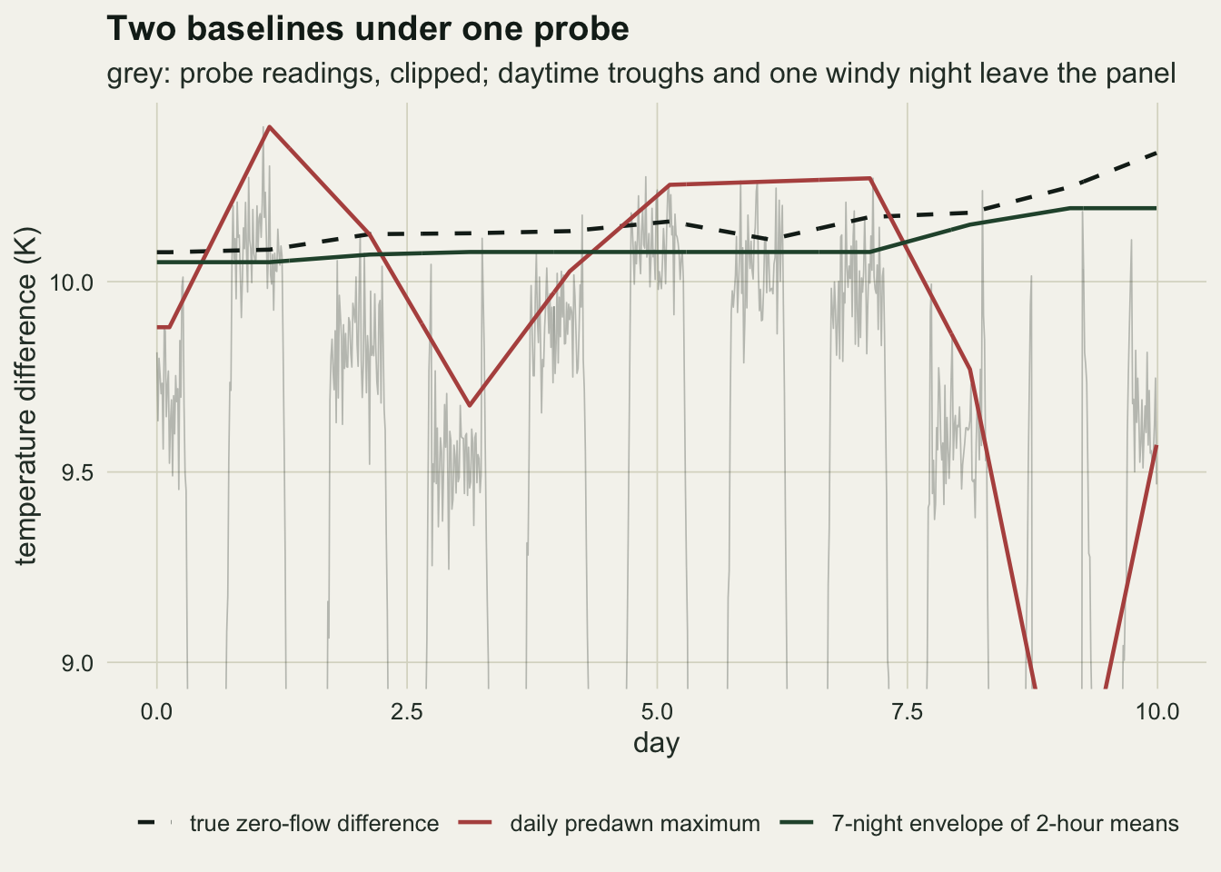
The grey trace is the probe, clipped so the night is visible: in daytime the difference falls as low as 6.1 K and leaves the panel. Calm nights in these ten days: 1. The predawn maximum jumps from night to night: above the dashed truth where a nearly still night lets the noise maximum show, below it where the night was windy, and off the bottom of the panel on the windiest night. The envelope of predawn means keeps the highest nightly value of the surrounding week and carries it across the windy nights, so it follows the truth from slightly below.
Two errors whose size is arithmetic
A constant night flow and no noise make the predawn maximum wrong by a fixed amount. Write K for the Granier flow index at zero-flow difference T0. At night the reading is T0 divided by one plus the night index, so the estimated baseline is exactly that, and every daytime index is shrunk to the true index minus the night index, divided by one plus the night index. Night flow itself is read as zero. This is algebra, and a loop over the day gives the monthly ratio without simulating anything.
predict_night <- function(fn, peak = u_peak, divide = TRUE) {
  u_d   <- pmax(peak * shape_day[1:96], fn * peak * is_night[1:96])
  k_d   <- (u_d / alpha_g)^(1 / beta_g)
  k_n   <- (fn * peak / alpha_g)^(1 / beta_g)
  u_est <- alpha_g * pmax((k_d - k_n) / (if (divide) 1 + k_n else 1), 0)^beta_g
  sum(u_est) / sum(u_d)
}
fn_check <- c(0, 0.025, 0.05, 0.1, 0.15, 0.2)
set.seed(3108)
check_night <- data.frame(fn = fn_check,
  predicted = sapply(fn_check, predict_night),
  simulated = sapply(fn_check, function(f) {
    s <- simulate_trees(5, f, 0, 0, wander = 0, cv = 0, vpd_const = TRUE)
    mean(score_rules(s, windows = 7)$ratio[, "predawn_max"])
  }))
gap_night <- max(abs(check_night$predicted - check_night$simulated))
r_10 <- check_night$predicted[check_night$fn == 0.1]
r_05 <- check_night$predicted[check_night$fn == 0.05]
r_20 <- check_night$predicted[check_night$fn == 0.2]
u_d10 <- pmax(u_peak * shape_day[1:96], 0.1 * u_peak * is_night[1:96])
night_share <- sum(0.1 * u_peak * is_night[1:96]) / sum(u_d10)
r_10_day <- r_10 / (1 - night_share)
idx_share <- 0.1^(1 / beta_g)
peak_set <- c(5, 15, 40); abs_set <- c(7.5, 15, 30)
r_peak   <- sapply(peak_set, function(p) predict_night(0.1, p))
r_nodiv  <- sapply(peak_set, function(p) predict_night(0.1, p, divide = FALSE))
r_abs    <- sapply(abs_set, function(p) predict_night(1.5 / p, p))
The prediction and the simulation differ by at most 3.39e-15 over the six night flow levels, which is rounding. A steady night flow of 5 per cent of the daytime peak gives 0.740 of the true monthly water use, 10 per cent gives 0.576 and 20 per cent gives 0.362. These numbers belong to this diurnal shape, this peak flux and this way of scaling night flow. Of the 0.424 lost at 10 per cent, 0.152 is the night flow itself, which the rule defines as zero; the rest is daytime flux read too low, and the daytime alone comes out at 0.680 of its truth. The exponent makes the daytime loss larger than a plain subtraction of the night flow would: the night index is the night flow share raised to 1/1.231, which is 0.154 of the peak index at 10 per cent rather than a tenth, and subtracting it bites hardest on the small indices of morning and evening. The peak enters only through the division by one plus the night index. With night flow held at 10 per cent of the peak, peaks of 5, 15 and 40 cm3 per cm2 per hour give 0.603, 0.576 and 0.527, and without that division all three would give 0.623. With the same absolute night flow of 1.5 cm3 per cm2 per hour, peaks of 7.5, 15 and 30 give 0.383, 0.576 and 0.716: a tree with a lower daytime peak loses a larger share. The numbers are consistent with the warning in Regalado and Ritter 2007 that a small night flow produces a large daytime error, and they are not a result of the simulation.
Noise alone has an arithmetic answer too. With no night flow the true predawn difference is constant, so the maximum of the twenty-four predawn readings exceeds it by the noise standard deviation times the expected maximum of twenty-four standard normal draws. That expectation is an integral, and plugging the raised baseline into the noise-free day gives a prediction.
e_max <- function(n) integrate(function(x) n * x * dnorm(x) * pnorm(x)^(n - 1), -Inf, Inf)$value
e_24  <- e_max(sum(is_pre[1:96]))
predict_noise <- function(noise_sd) {
  u_d <- u_peak * shape_day[1:96]
  dT0 <- dtmax0 / (1 + (u_d / alpha_g)^(1 / beta_g))
  sum(flux_from(dtmax0 + noise_sd * e_24, dT0)) / sum(u_d)
}
sd_check <- c(0.01, 0.03, 0.05, 0.1, 0.15)
set.seed(3109)
check_noise <- do.call(rbind, lapply(sd_check, function(s_n) {
  sc <- score_rules(simulate_trees(n_tree, 0, 0, s_n, wander = 0, cv = 0), windows = 7)$ratio
  data.frame(noise_sd = s_n, predicted = predict_noise(s_n),
             simulated = mean(sc[, "predawn_max"]),
             mc_se = sd(sc[, "predawn_max"]) / sqrt(n_tree),
             true_base = mean(sc[, "true_base"]))
}))
cn_03 <- check_noise[check_noise$noise_sd == 0.03, ]
cn_10 <- check_noise[check_noise$noise_sd == 0.1, ]
gap_10 <- cn_10$simulated - cn_10$predicted
The expected maximum of twenty-four standard normals is 1.95, so at a noise standard deviation of 0.03 K the predawn maximum sits 0.058 K too high on average. The prediction is 1.042 of true water use against a simulated 1.043; at 0.1 K it is 1.151 against 1.156 (Monte Carlo standard error 0.0006). The prediction leaves out the noise on the readings themselves. With the true baseline and noisy readings the ratio is 1.009 at 0.1 K, the same order as the gap of 0.005 between prediction and simulation: noise on a reading near zero flow is clipped at zero on one side and raised to the power 1.231 on the other, so it adds a little flow at night. That too is a property of the formula.
p_night <- ggplot(check_night, aes(100 * fn, predicted)) +
  geom_hline(yintercept = 1, linetype = "dashed", colour = te_ink, linewidth = 0.4) +
  geom_line(colour = te_rust, linewidth = 0.9) +
  geom_point(aes(y = simulated), colour = te_rust, size = 2.6) +
  labs(x = "steady night flow, per cent of peak", y = "estimated / true water use",
       title = "Night flow, no noise") +
  theme_datasheet()
p_noise <- ggplot(check_noise, aes(noise_sd, predicted)) +
  geom_hline(yintercept = 1, linetype = "dashed", colour = te_ink, linewidth = 0.4) +
  geom_line(colour = te_gold, linewidth = 0.9) +
  geom_point(aes(y = simulated), colour = te_gold, size = 2.6) +
  labs(x = "noise standard deviation (K)", y = "estimated / true water use",
       title = "Noise, no night flow") +
  theme_datasheet()
(p_night | p_noise) + plot_annotation(theme = theme_datasheet())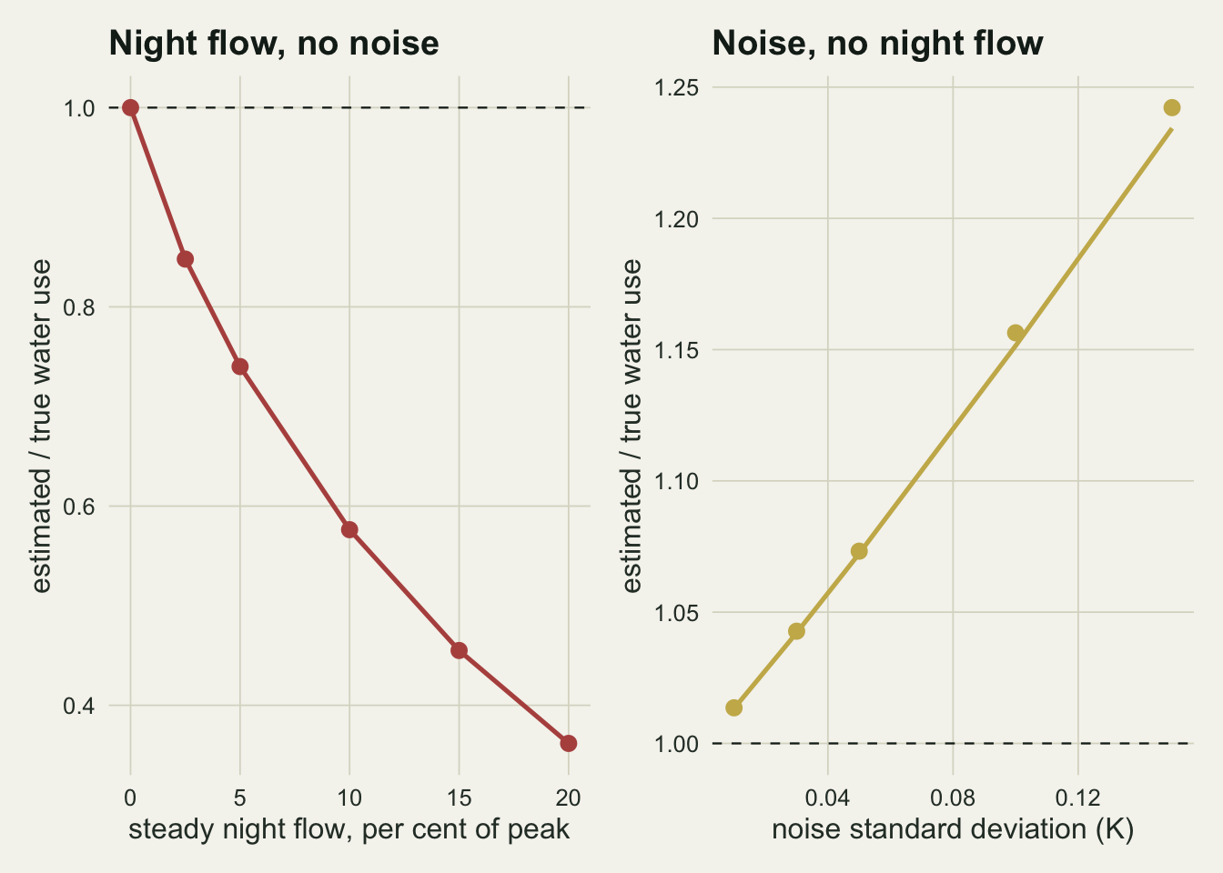
When night flow changes from night to night
Real nights differ, and that is where the rules separate. The predawn maximum takes each night as it comes, so it is wrong by that night’s flow. A multi-night envelope and the low deficit rule both depend on calm nights: when one falls inside the window, its baseline is carried to the windy nights around it. The share of calm nights is a property of the site and the month, not of the method, so it is swept here rather than chosen, at a night flow scale of 10 per cent and two noise levels.
calm_set  <- c(0, 0.1, 0.25, 0.5, 0.75)
sd_set    <- c(0.03, 0.1)
rules_show <- c(predawn_max = "daily predawn maximum", env_max_7 = "7-night envelope",
                low_vpd = "low deficit nights", env_mean_7 = "7-night envelope of 2-hour means")
set.seed(3110)
calm_cells <- expand.grid(calm = calm_set, noise_sd = sd_set)
calm_res <- do.call(rbind, lapply(seq_len(nrow(calm_cells)), function(i) {
  sc <- score_rules(simulate_trees(n_tree, fn_main, calm_cells$calm[i], calm_cells$noise_sd[i]),
                    windows = 7)
  out <- data.frame(calm = calm_cells$calm[i], noise_sd = calm_cells$noise_sd[i],
             rule = names(rules_show),
             ratio = colMeans(sc$ratio[, names(rules_show)]),
             mc_se = apply(sc$ratio[, names(rules_show)], 2, sd) / sqrt(n_tree),
             n_fall = sc$n_fall, gap = NA, gap_se = NA)
  m <- colMeans(sc$ratio[, names(rules_show)]); o <- order(abs(m - 1))
  g <- sign(m[o[2]] - 1) * sc$ratio[, names(rules_show)[o[2]]] -
       sign(m[o[1]] - 1) * sc$ratio[, names(rules_show)[o[1]]]
  out$gap <- abs(m[o[2]] - 1) - abs(m[o[1]] - 1); out$gap_se <- sd(g) / sqrt(n_tree)
  out
}))
get_r <- function(rule, calm, s_n) calm_res$ratio[calm_res$rule == rule & calm_res$calm == calm &
                                                  calm_res$noise_sd == s_n]
pre_lo <- min(calm_res$ratio[calm_res$rule == "predawn_max"])
pre_hi <- max(calm_res$ratio[calm_res$rule == "predawn_max"])
env_10 <- sapply(c(0, 0.25, 0.5), function(p) get_r("env_max_7", p, 0.1))
env_03 <- sapply(c(0, 0.25, 0.5), function(p) get_r("env_max_7", p, 0.03))
low_10 <- sapply(c(0, 0.25, 0.5), function(p) get_r("low_vpd", p, 0.1))
mean_10 <- sapply(c(0, 0.25, 0.5), function(p) get_r("env_mean_7", p, 0.1))
mean_03 <- sapply(c(0, 0.25, 0.5), function(p) get_r("env_mean_7", p, 0.03))
se_max <- max(calm_res$mc_se)
fall_max <- max(calm_res$n_fall)
p_below_thr <- pexp(vpd_thr, 1 / vpd_mean)
cell_split <- split(calm_res, list(calm_res$calm, calm_res$noise_sd))
best_rule <- sapply(cell_split, function(d) d$rule[which.min(abs(d$ratio - 1))])
decided <- sapply(cell_split, function(d) d$gap[1] > 2 * d$gap_se[1])
n_tie <- sum(!decided); gap_ratio_min <- min(sapply(cell_split[decided], function(d) d$gap[1] / d$gap_se[1]))
tie_txt <- paste(sapply(cell_split[!decided], function(d) {
  o <- order(abs(d$ratio - 1))
  sprintf("%s against %s at %.0f per cent calm nights and %.2f K, a gap of %.4f with standard error %.4f",
          rules_show[d$rule[o[1]]], rules_show[d$rule[o[2]]], 100 * d$calm[1], d$noise_sd[1],
          d$gap[1], d$gap_se[1])
}), collapse = "; ")
best_d <- best_rule[decided]
n_best_mean <- sum(best_d == "env_mean_7"); n_best_low <- sum(best_d == "low_vpd")
n_best_env <- sum(best_d == "env_max_7"); n_cells <- length(best_rule); n_dec <- sum(decided)
n_best_pre <- sum(best_d == "predawn_max")
best_03 <- best_d[grepl("0.03$", names(best_d))]; best_10 <- best_d[grepl("0.1$", names(best_d))]
n_low_03 <- sum(best_03 == "low_vpd"); n_mean_10 <- sum(best_10 == "env_mean_7")
pre_75_10 <- get_r("predawn_max", 0.75, 0.1)
low_03_lo <- min(calm_res$ratio[calm_res$rule == "low_vpd" & calm_res$noise_sd == 0.03])
low_03_hi <- max(calm_res$ratio[calm_res$rule == "low_vpd" & calm_res$noise_sd == 0.03])
mean_10_lo <- min(calm_res$ratio[calm_res$rule == "env_mean_7" & calm_res$noise_sd == 0.1])
mean_10_hi <- max(calm_res$ratio[calm_res$rule == "env_mean_7" & calm_res$noise_sd == 0.1])calm_res$rule_lab <- factor(rules_show[calm_res$rule], levels = rules_show)
calm_res$noise_lab <- factor(sprintf("noise sd %.2f K", calm_res$noise_sd))
ggplot(calm_res, aes(100 * calm, ratio, colour = rule_lab)) +
geom_hline(yintercept = 1, linetype = "dashed", colour = te_ink, linewidth = 0.4) +
geom_line(linewidth = 0.9) + geom_point(size = 2.2) +
facet_wrap(~ noise_lab) +
scale_colour_manual(values = c(te_rust, te_gold, te_ink, te_forest), name = NULL) +
labs(x = "calm nights (per cent)", y = "estimated / true water use",
title = "No rule is right for every month") +
guides(colour = guide_legend(nrow = 2)) +
theme_datasheet() + theme(legend.position = "bottom")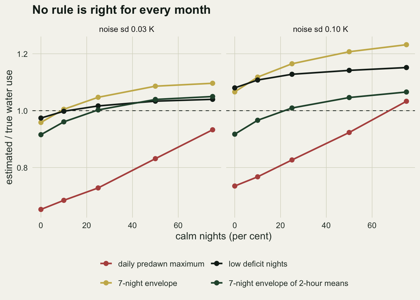
Across the whole grid the daily predawn maximum returns between 0.653 and 1.033 of the true thirty-day water use. It is low in every cell but one, and that one is not a success: at 75 per cent calm nights and 0.1 K of noise it reads 1.033 because the noise maximum on the calm nights happens to outweigh the flow on the others. The largest Monte Carlo standard error of any mean in the figure is 0.0049, so gaps of a few hundredths between the lines are real. Where two lines nearly cross, the order is not: the gap between the nearest and the second nearest rule is compared below with its paired standard error over the trees.
The seven-night envelope of the predawn maxima does recover the night flow, and then goes past it. At 0.1 K of noise it reads 1.066, 1.165 and 1.207 with no calm nights, a quarter and a half; at 0.03 K the same cells read 0.959, 1.047 and 1.086. The more calm nights there are, the more often the envelope finds a baseline with no flow under it, and what it then carries forward is the largest of seven noisy maxima rather than the truth. Even the cell with no calm nights is not free of low-flow nights: an exponential deficit with mean 0.5 kPa falls below 0.1 kPa on 18 per cent of windy nights, which is why the envelope gets close to one there at low noise.
The low deficit rule behaves the same way, with a smaller overshoot once calm nights are common, because it takes the maximum only on qualifying nights and interpolates between them instead of taking a running maximum: at 0.1 K it reads 1.080, 1.128 and 1.142. At 0.03 K of noise it stays between 0.974 and 1.040 over all five calm shares. It needed the envelope as a fallback for at most 4 of the 150 trees in any cell. It also had something no field record has, the deficit of each night measured without error.
The rule that changes the picture is the envelope of 2-hour means: the same seven-night window, but over the mean of the last eight predawn readings rather than their maximum. At 0.1 K of noise it reads 0.917, 1.009 and 1.046, and over all five calm shares it stays between 0.917 and 1.066. Counting which rule lands nearest to one, ties come first. In 1 of the 10 cells the gap is within two standard errors: low deficit nights against 7-night envelope at 10 per cent calm nights and 0.03 K, a gap of 0.0028 with standard error 0.0044. In the other 9 cells the gap is at least 3.5 standard errors, and the envelope of means wins 4, the low deficit rule 3, the plain envelope 1 and the predawn maximum 1, the cell where its two errors cancel. The ranking turns with the noise: at 0.03 K the low deficit rule is nearest in 3 of the 4 calm shares that are not ties, at 0.1 K the envelope of means in 3 of 5. It belongs to these design constants, not to sap flow in general.
The envelope window trades night flow for noise
A longer window is more likely to contain a calm night, which pulls the baseline up towards the truth. It also takes the maximum over more readings, which pulls it past the truth by the noise, and over more days of a wandering zero, which does the same. The window sweep below holds the calm share at 25 per cent and the noise at 0.1 K and changes the night flow scale.
fn_set <- c(0, 0.05, 0.1, 0.2)
win_set <- c(3, 7, 11)
set.seed(3111)
win_res <- do.call(rbind, lapply(fn_set, function(f) {
  rt <- colMeans(score_rules(simulate_trees(n_tree, f, calm_main, sd_main), windows = win_set)$ratio)
  rbind(data.frame(fn = f, window = c(1, win_set), stat = "maximum of the readings",
                   ratio = unname(rt[c("predawn_max", paste0("env_max_", win_set))])),
        data.frame(fn = f, window = c(1, win_set), stat = "mean of 04:00 to 06:00",
                   ratio = unname(rt[c("predawn_mean", paste0("env_mean_", win_set))])))
}))
get_w <- function(f, wd, st) win_res$ratio[win_res$fn == f & win_res$window == wd & win_res$stat == st]
max_st <- "maximum of the readings"; mean_st <- "mean of 04:00 to 06:00"
w0_max  <- sapply(c(1, 3, 7, 11), function(wd) get_w(0, wd, max_st))
w0_mean <- sapply(c(1, 3, 7, 11), function(wd) get_w(0, wd, mean_st))
w20_max  <- sapply(c(1, 3, 7, 11), function(wd) get_w(0.2, wd, max_st))
w20_mean <- sapply(c(1, 3, 7, 11), function(wd) get_w(0.2, wd, mean_st))
w7_max  <- range(win_res$ratio[win_res$window == 7 & win_res$stat == max_st])
w7_mean <- range(win_res$ratio[win_res$window == 7 & win_res$stat == mean_st])
set.seed(3112)
still <- colMeans(score_rules(simulate_trees(n_tree, 0, calm_main, sd_main, wander = 0),
                              windows = 7)$ratio)
wander_add_mean <- w0_mean[3] - still["env_mean_7"]; wander_add_max <- w0_max[3] - still["env_max_7"]win_res$fn_lab <- factor(sprintf("%.0f per cent", 100 * win_res$fn),
levels = sprintf("%.0f per cent", 100 * fn_set))
ggplot(win_res, aes(window, ratio, colour = fn_lab)) +
geom_hline(yintercept = 1, linetype = "dashed", colour = te_ink, linewidth = 0.4) +
geom_line(linewidth = 0.9) + geom_point(size = 2.2) +
facet_wrap(~ stat) +
scale_x_continuous(breaks = c(1, 3, 7, 11)) +
scale_colour_manual(values = c(te_ink, te_gold, te_forest, te_rust), name = "night flow scale") +
labs(x = "envelope window (nights)", y = "estimated / true water use",
title = "Longer windows find calm nights and noise") +
theme_datasheet() + theme(legend.position = "bottom")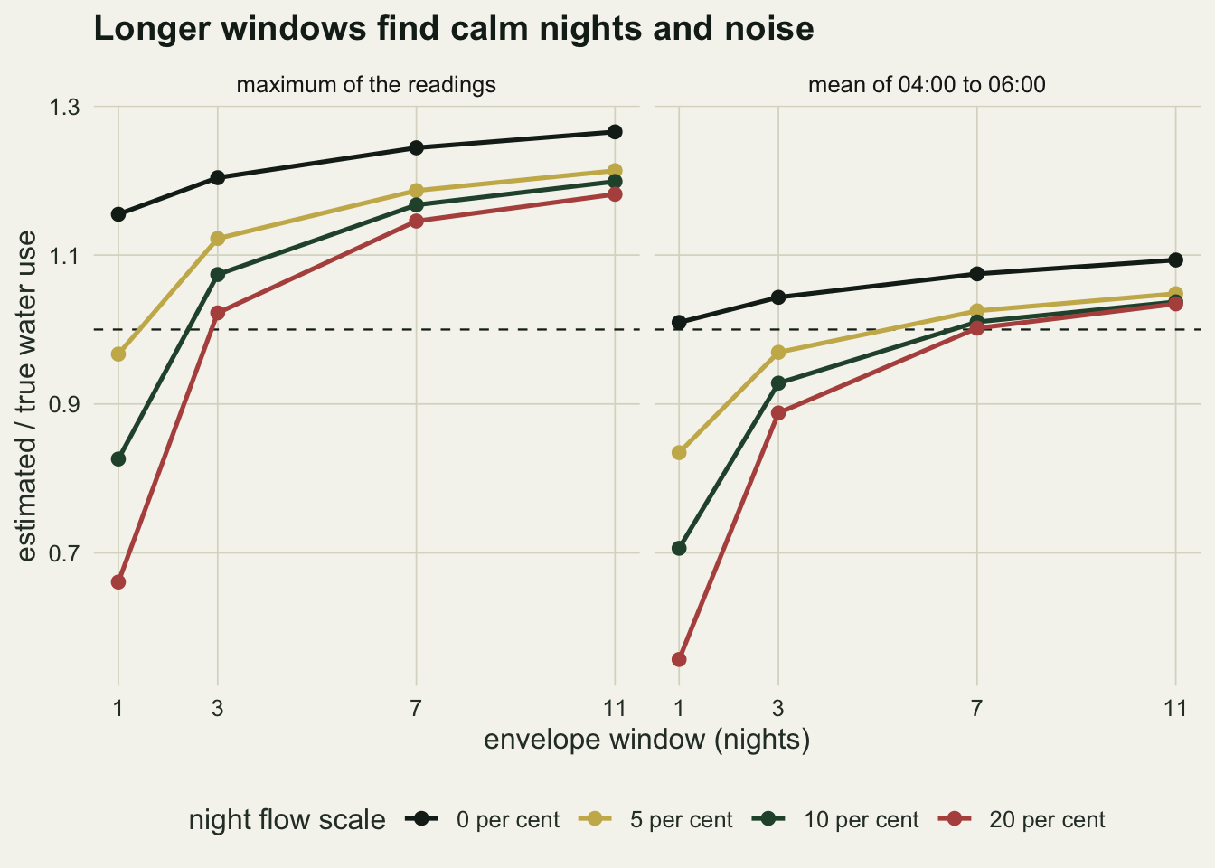
With no night flow at all, the left panel is pure noise and wander. The daily predawn maximum reads 1.155, and widening the window to 3, 7 and 11 nights raises it to 1.204, 1.244 and 1.265. The same windows over the 2-hour means give 1.010, 1.043, 1.075 and 1.093. Most of the noise part has gone, but not all of it, and the zero itself wanders. With the wander switched off, the seven-night envelope of means reads 1.040 and the seven-night envelope of maxima 1.215, so the wander adds 0.035 and 0.029 to them. What remains in the envelope of means is the largest of seven nightly means, each of which carries the noise of eight readings rather than one, plus the small inflation that noisy readings cause with a perfect baseline.
At a night flow scale of 20 per cent the daily rule is far off and every window helps. The maximum reads 0.661 at one night and 1.022, 1.146 and 1.182 at 3, 7 and 11; the mean reads 0.557, then 0.888, 1.002 and 1.034. At one night, averaging makes things worse: a 2-hour mean is lower than the maximum of the same night, and in the daily rule the noise maximum was partly cancelling the night flow. Averaging pays only once a window is there to find the calm nights.
The practical reading is the spread at a fixed window across night flow scales the analyst does not know. At seven nights, over the four scales, the envelope of maxima runs from 1.146 to 1.244 and the envelope of means from 1.002 to 1.075. The second is both closer to one and narrower, and neither depends on knowing how much the tree transpired at night.
A daily value is less certain than a monthly sum
daily_q <- sapply(sc_main$daily[c("predawn_max", "env_max_7", "env_mean_7")],
                  function(m) quantile(m, c(0.05, 0.5, 0.95)))
month_q <- sapply(c("predawn_max", "env_max_7", "env_mean_7"),
                  function(r) quantile(sc_main$ratio[, r], c(0.05, 0.95)))
Everything above is a thirty-day sum, and a sum over a month lets errors on different days cancel. In the cell of the first figure (10 per cent night flow scale, a quarter calm nights, 0.1 K of noise) the daily ratio of estimated to true water use under the envelope of 2-hour means has a 5 to 95 per cent range of 0.877 to 1.125 over all trees and days, while the 5 to 95 per cent range of the thirty-day ratio of individual trees is 0.953 to 1.057. Under the daily predawn maximum the daily range is 0.428 to 1.168, and under the plain seven-night envelope 1.019 to 1.337. A study that relates daily water use to daily weather inherits the daily spread, and part of that spread can be correlated with the weather, because under the daily rule a windy night lowers the baseline for the days on both sides of it. Peters and colleagues 2018 report that zero-flow conditions ignoring night-time water use reduced the correlation between environment and sap flux density. The simulation here draws the night deficit independently of daytime demand, so it does not show this.
What to report
Name the baseline rule in full: which readings enter the nightly value (the maximum, or a mean over which hours), the window in nights, any environmental filter with its threshold, and whether the baseline was edited by hand. At one night flow scale, the rules compared here put the thirty-day water use anywhere from 0.653 to 1.232 of the truth, so a water use number without the rule is not interpretable.
State the logging interval and the noise of the probe, estimated from the scatter of predawn readings on calm nights. The noise sets the overshoot of every rule that takes a maximum, and its size can be predicted from the expected maximum of the number of readings that the rule scans.
If night-time deficit or wind is measured on site, report the share of nights that met the low-flow criterion in each month. That share decides whether an envelope or a filtered baseline can recover the zero at all, and it is the quantity the reader needs to judge the months where it was low.
When the result is a sum over weeks, a baseline that is right on average is enough. When it is a daily series related to daily weather, say so and show the daily scatter of the baseline itself, because a baseline that dips around windy nights can put the weather into the response.
If night-time transpiration is itself a result of the study, the predawn maximum cannot be used: it defines night flow as zero on the very nights that are being measured.
Honest limits
The generating model is simple on purpose and several of its choices carry the numbers. The daytime shape, the peak flux and the Granier coefficients set how hard a given baseline error bites, and the arithmetic section shows that the loss from a steady night flow depends on them directly. A tree with a lower daytime peak and the same absolute night flow, or a species whose true calibration differs from Granier’s, would put every line in a different place. Species-specific calibration is out of scope here, and in the conifer data of Peters and colleagues 2018 working without site- and species-specific calibration lowered their whole-tree water use estimates by 37 per cent.
Night flow here is transpiration driven by the night deficit and nothing else. Real stems also refill their storage after a dry day, which produces flow at the probe on nights with no deficit and decays towards dawn; a calm night after a dry day is then not a zero-flow night, and every rule that relies on calm nights is fooled by it. Separating refilling from night transpiration needs measurements this post does not have.
The probe error is Gaussian white noise plus a slow wander of the zero. Natural temperature gradients in the stem, which shift the difference with the probe heater off, sensor drift over a season, and wounding are not in the model; nor is the radial profile of flux in the sapwood. The deficit is known without error and so is the calm-night state, which flatters the low deficit rule.
The envelope rule is a running maximum, not Baseliner and not the optimisation in Regalado and Ritter 2007. Baseliner combines automatic filters with inspection by eye, and a person who looks at the trace would catch the worst windy nights in a way no rule here does. The comparison is between simple, fully automatic rules, which is what a script applied to hundreds of probes does.
Finally, each cell uses 150 trees with independent noise and independent weather. In a stand the trees share their nights, so calm nights come in the same weeks for every probe and the stand total does not average out the baseline error the way the mean over simulated trees does.
References
Granier A 1985 Annales des Sciences Forestieres 42(2):193-200 (10.1051/forest:19850204)
Regalado CM, Ritter A 2007 Tree Physiology 27(8):1093-1102 (10.1093/treephys/27.8.1093)
Oishi AC, Hawthorne DA, Oren R 2016 SoftwareX 5:139-143 (10.1016/j.softx.2016.07.003)
Peters RL, Fonti P, Frank DC, Poyatos R, Pappas C, Kahmen A, et al 2018 New Phytologist 219(4):1283-1299 (10.1111/nph.15241)