Night-time flux and the u-star threshold

A simulated year of half-hourly eddy covariance data measures the friction velocity filter: what it recovers, what it discards and what it costs a budget.

A flux tower stands on a temperate fen at forty-seven degrees north, sonic anemometer and gas analyser on a short mast a couple of metres above a sedge canopy. It has been running for a year. The logger writes one record every half hour, so the year is seventeen thousand five hundred and twenty rows of net ecosystem exchange, air and soil temperature, incoming radiation and friction velocity. The question the tower was put up to answer is whether the fen took up carbon over the year and how much.

The sign convention first, because it causes more confusion than anything else here. Net ecosystem exchange is written from the atmosphere’s point of view: a negative flux is carbon leaving the air and entering the ecosystem, a positive flux is carbon going the other way. So daytime half hours in the growing season are negative, every night-time half hour is positive, and an annual sum that comes out negative describes a sink.

Eddy covariance works by measuring the covariance between vertical wind speed and gas concentration, which means it needs vertical wind. On a calm clear night there is very little. The air near the ground stratifies, turbulence collapses, and the carbon dioxide respired by the soil and the plants does not reach the sensor: it pools in the canopy air below it, or drains sideways down whatever slope exists, and is measured hours later or not at all. Goulden et al (1996) set this out in the first careful accuracy audit of a long eddy covariance record, and the standard response has been the same ever since: measure the friction velocity, decide on a threshold below which the night-time flux is not to be trusted, and throw those half hours away. This post simulates a year in which the true flux is known at every half hour, applies that attenuation, and runs the estimator practitioners use, to see how close it gets, what it costs in data and what it does to the annual number.

What this post is and is not next to

The nearest neighbour on this site is the litter decomposition cluster, and the difference is worth stating because the two look superficially similar and fail in completely different ways. Mass loss and the carbon budget also converts a measurement into a carbon flux, but there the measurement is a bag on a balance: a discrete object, weighed on eight occasions over five years, with corrections that are multiplicative and systematic, to do with what the mass is made of and what fell into the bag. Here nothing is weighed and the year is an integral of seventeen thousand half hours. The failure mode is not a wrong conversion factor applied to a correct number; it is a subset of the record, selected by weather rather than at random, in which the instrument was reading low, plus the decision about which subset that was.

This is the first of four posts on eddy covariance. This one stops at the threshold: it estimates it, prices it and leaves gaps in the record. Filling those gaps is gap filling a flux time series; splitting the filled record into gross primary production and ecosystem respiration is partitioning net flux into GPP and respiration; auditing the finished figure is checking an annual flux budget.

library(ggplot2)

te_pal <- list(forest = "#275139", green = "#2f8f63", sage = "#93a87f",
               clay = "#b5534e", gold = "#cda23f", line = "#dad9ca",
               ink = "#16241d", paper = "#f5f4ee")

theme_te <- function() {
  theme_minimal(base_size = 12) +
    theme(panel.grid.minor = element_blank(),
          panel.grid.major = element_line(colour = "#e7e6dc"),
          plot.background = element_rect(fill = "#f5f4ee", colour = NA),
          panel.background = element_rect(fill = "#f5f4ee", colour = NA),
          plot.title = element_text(face = "bold", colour = te_pal$ink),
          axis.title = element_text(colour = "#2c3a31"),
          axis.text = element_text(colour = "#2c3a31"))
}

A year of half hours

The drivers come first: solar geometry from latitude and day of year, cloudiness as a day-to-day autocorrelated series, air temperature with a seasonal cycle, a diurnal cycle and synoptic wobble, and a soil temperature that is a damped and lagged version of it. One feature of the temperature field is put in deliberately and matters later. Daytime heating is stronger under clear skies and night-time cooling is too: on a clear night the surface loses heat to space, the loss accumulates, and the near-surface air and the top of the soil keep falling until dawn. That accumulation is written as a term in the square root of the hours since sunset, the usual shape for radiative cooling under a stable layer.

n_half <- 17520
tix <- seq_len(n_half)
doy <- (tix - 1) %/% 48 + 1
hod <- ((tix - 1) %% 48) * 0.5 + 0.25
lat_deg <- 47
declin <- 23.44 * sin(2 * pi * (284 + doy) / 365) * pi / 180
sin_elev <- sin(lat_deg * pi / 180) * sin(declin) +
  cos(lat_deg * pi / 180) * cos(declin) * cos((hod - 12) * 15 * pi / 180)
is_night <- sin_elev <= 0
rl <- rle(is_night)
hrs_dark <- 0.5 * sequence(rl$lengths) * rep(as.integer(rl$values), rl$lengths)
night_id <- (tix + 23) %/% 48 + 1

set.seed(20260802)
cloud <- plogis(as.numeric(stats::filter(rnorm(365, 0, 0.8), 0.62,
                                         method = "recursive")) - 0.15)
clear <- 1 - rep(cloud, each = 48)
ppfd <- pmax(0, 2100 * sin_elev) * (0.22 + 0.72 * clear)
seas_t <- 9 + 9.5 * sin(2 * pi * (doy - 112) / 365)
syn <- rep(as.numeric(stats::filter(rnorm(365, 0, 1.7), 0.72,
                                    method = "recursive")), each = 48)
anom <- (2 + 7 * clear) * pmax(0, sin_elev) - 2.1 * clear * sqrt(hrs_dark)
tair <- seas_t + syn + anom
ts_slow <- as.numeric(stats::filter(0.004 * (seas_t + syn), 0.996,
                                    method = "recursive",
                                    init = seas_t[1] + syn[1]))
tsoil <- ts_slow + 0.42 * anom

print(round(c(half_hours = n_half, nights = max(night_id),
              night_fraction = mean(is_night),
              longest_night_hours = max(hrs_dark)), 3))

         half_hours              nights      night_fraction longest_night_hours 
            17520.0               366.0                 0.5                16.0 

print(round(c(air_min = min(tair), air_max = max(tair),
              soil_min = min(tsoil), soil_max = max(tsoil),
              peak_light = max(ppfd)), 2))

   air_min    air_max   soil_min   soil_max peak_light 
     -8.94      28.50      -4.42      22.40    1592.51 

The record covers 17520 half hours over 366 nights, and 50 per cent of it falls with the sun below the horizon, the longest night running to 16 hours. Air temperature spans -8.9 to 28.5 degrees C and soil temperature -4.4 to 22.4, with peak photosynthetic photon flux density of 1593 umol/m2/s.

The true fluxes are built from two standard response functions. Ecosystem respiration follows the temperature response of Lloyd and Taylor (1994), driven by soil temperature, and gross primary production follows a rectangular hyperbola in light whose asymptote is scaled by a seasonal greenness curve. Net ecosystem exchange is respiration minus production, so it is positive at night and negative in the middle of a summer day.

r_ref <- 2.2
e0_lt <- 300
reco <- r_ref * exp(e0_lt * (1 / (283.15 - 227.13) -
                               1 / ((tsoil + 273.15) - 227.13)))
green <- 1 / (1 + exp(-(doy - 108) / 11)) * 1 / (1 + exp((doy - 288) / 14))
green <- 0.02 + 0.98 * green
a_max <- 18 * green
alph <- 0.038
gpp <- a_max * alph * ppfd / (a_max + alph * ppfd)
gpp[ppfd <= 0] <- 0
nee_true <- reco - gpp

conv <- 1800 * 12.011e-6
c_reco <- sum(reco) * conv
c_gpp <- sum(gpp) * conv
c_true <- sum(nee_true) * conv

print(round(c(reco_ref_umol = r_ref, activation_e0 = e0_lt,
              quantum_yield = alph, amax_peak = max(a_max)), 4))

reco_ref_umol activation_e0 quantum_yield     amax_peak 
       2.2000      300.0000        0.0380       17.9739 

print(round(c(annual_reco = c_reco, annual_gpp = c_gpp,
              annual_nee = c_true,
              night_mean_flux = mean(nee_true[is_night]),
              day_min_flux = min(nee_true)), 3))

    annual_reco      annual_gpp      annual_nee night_mean_flux    day_min_flux 
        865.119        1096.581        -231.462           1.817          -9.273 

Over the year the fen respires 865 gC/m2 and fixes 1097 gC/m2, so the true net exchange is -231.46 gC/m2/yr, a sink of moderate size for a temperate peatland. Night-time flux averages 1.817 umol/m2/s and the strongest midsummer uptake reaches -9.27 umol/m2/s. That annual figure is the thing every method below is trying to recover, and in the field it does not exist.

The defect: what a calm night does to the measurement

Friction velocity is the square root of the momentum flux and it is the field measure of how much mechanical turbulence there is. The series here has four parts: a daytime convective boost that follows solar elevation, a synoptic wind component that persists for a few days at a time, a seasonal roughness term tied to the greenness curve, since a sedge canopy in July is rougher than the same fen in February, and a stability penalty on clear nights that deepens as the night goes on. The last two are what link turbulence to temperature. A clear calm night is both the least turbulent and the coldest; a windy cloudy one is neither. That link is physics rather than an artefact of the simulation, and it is why the estimator in the next section is more complicated than it first looks as though it needs to be.

set.seed(20260803)
w_syn <- rep(as.numeric(stats::filter(rnorm(365, 0, 0.32), 0.70,
                                      method = "recursive")), each = 48)
eps_u <- as.numeric(stats::filter(rnorm(n_half, 0, 0.11), 0.86,
                                  method = "recursive"))
ustar <- exp(log(0.40) + 0.55 * pmax(0, sin_elev)^0.6 + 0.32 * green + w_syn -
               0.55 * clear * is_night - 0.055 * clear * hrs_dark + eps_u)

u_mid <- 0.16
u_w <- 0.040
u_true <- u_mid + u_w * log(99)
att <- ifelse(is_night, plogis((ustar - u_mid) / u_w), 1)
nee_att <- nee_true * att

print(round(quantile(ustar[is_night], c(0.05, 0.25, 0.5, 0.75, 0.95)), 3))

   5%   25%   50%   75%   95% 
0.116 0.214 0.311 0.440 0.782 

print(round(c(ramp_midpoint = u_mid, ramp_width = u_w,
              true_threshold = u_true,
              transfer_at_midpoint = plogis(0),
              transfer_at_threshold = plogis((u_true - u_mid) / u_w)), 4))

        ramp_midpoint            ramp_width        true_threshold 
               0.1600                0.0400                0.3438 
 transfer_at_midpoint transfer_at_threshold 
               0.5000                0.9900 

print(round(c(mean_night_transfer = mean(att[is_night]),
              mean_flux_lost = mean(nee_true[is_night] - nee_att[is_night]),
              night_below_threshold = mean(ustar[is_night] < u_true),
              carbon_lost = sum(nee_true * (1 - att)) * conv), 4))

  mean_night_transfer        mean_flux_lost night_below_threshold 
               0.8473                0.2177                0.5811 
          carbon_lost 
              41.2389 

The attenuation is a logistic ramp in friction velocity rather than a step. Below a midpoint of 0.16 m/s more than half the respired carbon fails to reach the sensor; well above it the flux passes intact. Defining the true threshold as the friction velocity at which 99 per cent of the flux gets through puts it at 0.3438 m/s, and that is the number every estimate below is compared against. A step would make the estimation problem trivial and would also be wrong, since the collapse of turbulent transport is gradual.

Over the year 58.1 per cent of night-time half hours sit below that threshold, the average night-time half hour delivers 84.7 per cent of its true flux, and the carbon that never reaches the sensor totals 41.2 gC/m2 across the year. Measurement noise goes on top. Real flux noise is not constant: its scale grows with the size of the flux, as Richardson et al (2006) showed across a range of towers, so the standard deviation here is an offset plus a fraction of the flux magnitude.

set.seed(20260804)
sig <- 0.45 + 0.12 * abs(nee_att)
nee_obs <- nee_att + rnorm(n_half, 0, sig)
nu <- ustar[is_night]
nt <- tsoil[is_night]
nf <- nee_obs[is_night]
nid <- night_id[is_night]

print(round(c(noise_floor = 0.45, noise_slope = 0.12,
              mean_sigma = mean(sig), sigma_night = mean(sig[is_night]),
              sigma_day = mean(sig[!is_night])), 4))

noise_floor noise_slope  mean_sigma sigma_night   sigma_day 
     0.4500      0.1200      0.7506      0.6419      0.8592 

print(round(c(sd_night_flux = sd(nf), mean_night_flux = mean(nf),
              annual_sum_noise_sd = sqrt(sum(sig^2)) * conv), 4))

      sd_night_flux     mean_night_flux annual_sum_noise_sd 
             1.4728              1.5934              2.3037 

The noise standard deviation averages 0.751 umol/m2/s, against a night-time flux that averages 1.593 with a standard deviation of 1.473. Summed over the whole year the noise contributes a standard deviation of only 2.304 gC/m2/yr to the annual total, because seventeen thousand independent errors mostly cancel. Hold on to that figure; it is the yardstick the last section measures the threshold uncertainty against.

The fall-off is not visible in the record

The first thing to establish is that nothing in the time series announces the problem. A fortnight of summer half hours, with the badly attenuated ones marked, looks like a fortnight of ordinary flux data.

Figure 1: Twelve days of half-hourly net ecosystem exchange in late June as the logger recorded it. Negative values are daytime uptake, positive values are night-time release. Red points are the night-time half hours where the simulated attenuation removed more than a tenth of the true flux. They fall inside the ordinary night-to-night scatter and there is nothing in their position or their spacing to mark them out.

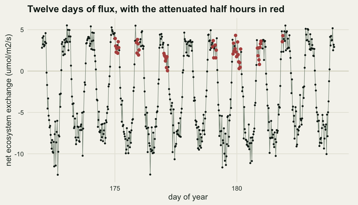
Two measurements say the same thing with numbers: the size of the loss against the size of the ordinary variation, and how much of the variance in night-time flux friction velocity accounts for, before and after soil temperature has been taken out of it.

loss_night <- mean(nee_true[is_night] - nee_att[is_night])
fit_t <- lm(nf ~ nt)
fit_u <- lm(nf ~ nu)
fit_p <- lm(residuals(fit_t) ~ nu)

nm_f <- as.numeric(tapply(nee_obs[is_night], nid, mean))
nm_u <- as.numeric(tapply(ustar[is_night], nid, mean))
calm <- nm_u < u_true
gap_nightly <- mean(nm_f[!calm]) - mean(nm_f[calm])

print(round(c(mean_flux_lost = loss_night, sd_night_flux = sd(nf),
              loss_over_sd = loss_night / sd(nf)), 4))

mean_flux_lost  sd_night_flux   loss_over_sd 
        0.2177         1.4728         0.1478 

print(round(c(r2_soil_temperature = summary(fit_t)$r.squared,
              r2_ustar = summary(fit_u)$r.squared,
              r2_ustar_after_temperature = summary(fit_p)$r.squared), 4))

       r2_soil_temperature                   r2_ustar 
                    0.6732                     0.1484 
r2_ustar_after_temperature 
                    0.0755 

print(round(c(calm_nights = sum(calm), other_nights = sum(!calm),
              mean_flux_calm = mean(nm_f[calm]),
              mean_flux_other = mean(nm_f[!calm]),
              apparent_gap = gap_nightly,
              actual_loss = loss_night,
              gap_over_loss = gap_nightly / loss_night), 4))

    calm_nights    other_nights  mean_flux_calm mean_flux_other    apparent_gap 
       187.0000        179.0000          1.2131          2.4618          1.2487 
    actual_loss   gap_over_loss 
         0.2177          5.7347 

The attenuation removes 0.2177 umol/m2/s from the average night-time half hour, against a night-time standard deviation of 1.473: a ratio of 0.148. Soil temperature accounts for 67.3 per cent of the variance in night-time flux and friction velocity for 14.8 per cent on its own, falling to 7.5 per cent once temperature has been removed first. Anyone looking at the record without a specific reason to bin it by turbulence will see temperature and nothing else.

The nightly aggregate makes the trap sharper. Averaging each night and splitting the 366 nights at the true threshold gives 187 calm nights averaging 1.213 umol/m2/s and 179 others averaging 2.462, an apparent gap of 1.249. That gap is 5.73 times the flux the attenuation actually removed. Most of it is temperature: calm nights are clear nights and clear nights are cold. A reader who took that gap for the size of the problem would be out by nearly a factor of six, in a direction that is not obvious.

The signature, and where it hides

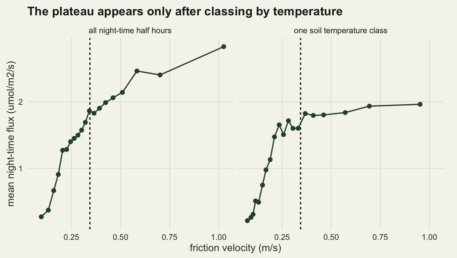
The way to see the attenuation is to sort the night-time half hours by friction velocity, cut them into equal-sized bins and take the mean flux in each. If turbulence is doing nothing to the measurement, the bin means are flat. If it is, they climb from the left and then level off, and the levelling-off point is the threshold. Aubinet et al (2000) made that plot part of the standard EUROFLUX processing chain and it has been the diagnostic ever since.

bin_table <- function(us, fx, tp, n_bin = 20) {
  bn <- cut(us, quantile(us, seq(0, 1, length.out = n_bin + 1)),
            include.lowest = TRUE, labels = FALSE)
  data.frame(bin = seq_len(n_bin),
             ustar = as.numeric(tapply(us, bn, mean)),
             flux = as.numeric(tapply(fx, bn, mean)),
             soil = as.numeric(tapply(tp, bn, mean)),
             n = as.numeric(table(bn)))
}

pool_tab <- bin_table(nu, nf, nt)
t_class <- cut(nt, quantile(nt, seq(0, 1, length.out = 7)),
               include.lowest = TRUE, labels = FALSE)
in_cls <- which(t_class == 4)
cls_tab <- bin_table(nu[in_cls], nf[in_cls], nt[in_cls])

print(round(pool_tab[c(1, 4, 8, 12, 16, 20), ], 3))

   bin ustar  flux   soil   n
1    1 0.096 0.272  5.490 438
4    4 0.183 0.908  4.185 438
8    8 0.264 1.451  5.395 438
12  12 0.341 1.864  6.845 438
16  16 0.462 2.061  7.705 438
20  20 1.025 2.828 12.160 438

print(round(cls_tab[c(1, 4, 8, 12, 16, 20), ], 3))

   bin ustar  flux  soil  n
1    1 0.073 0.214 7.842 73
4    4 0.114 0.511 8.082 73
8    8 0.189 1.131 7.842 73
12  12 0.282 1.715 7.635 73
16  16 0.408 1.795 8.135 73
20  20 0.952 1.962 9.026 73

print(round(c(pooled_soil_range = diff(range(pool_tab$soil)),
              class_soil_range = diff(range(cls_tab$soil)),
              pooled_flux_low = pool_tab$flux[1],
              pooled_flux_high = mean(pool_tab$flux[16:20]),
              class_flux_low = cls_tab$flux[1],
              class_flux_high = mean(cls_tab$flux[16:20])), 3))

pooled_soil_range  class_soil_range   pooled_flux_low  pooled_flux_high 
            8.608             1.422             0.272             2.379 
   class_flux_low   class_flux_high 
            0.214             1.867 

Pooling every night-time half hour in the year gives a curve that rises across the whole range, from 0.272 umol/m2/s in the lowest bin to 2.379 in the top five, and never plateaus. The soil temperature column says why: mean soil temperature in the pooled bins spans 8.61 degrees C, because the seasonal roughness of the canopy has loaded the high friction velocity bins with summer nights, so the curve is measuring the season as much as the turbulence. Restricting to one of six soil temperature classes shrinks that spread to 1.42 degrees C and the shape changes: the flux climbs from 0.214 umol/m2/s to a plateau at 1.867 and stops. That is the signature, and temperature classing is what makes it appear.

Figure 2: Mean night-time flux in twenty equal-sized friction velocity bins, pooled over the whole year on the left and within a single soil temperature class on the right. The dashed vertical line is the true threshold used to generate the data. The pooled curve rises across the entire range and never plateaus, because the friction velocity bins differ in season and therefore in temperature. Inside one temperature class the plateau appears where it should.

The moving point test

The estimator in general use is the moving point test of Gu et al (2005), in the form standardised by Papale et al (2006). Split the night-time record into temperature classes. Inside each class, sort by friction velocity and cut into twenty equal-sized bins. Walk up the bins and take the first one whose mean flux reaches ninety-nine per cent of the mean of all the bins above it: that bin’s friction velocity is the class threshold. Discard any class in which friction velocity and temperature are correlated beyond a set limit, on the grounds that the classing has failed there. Take the median of what is left.

mpt_bin <- function(us, fx, n_bin = 20, crit = 0.99) {
  if (length(us) < 5 * n_bin) return(NA_real_)
  bn <- cut(us, quantile(us, seq(0, 1, length.out = n_bin + 1)),
            include.lowest = TRUE, labels = FALSE)
  m_f <- as.numeric(tapply(fx, bn, mean))
  m_u <- as.numeric(tapply(us, bn, mean))
  for (i in seq_len(n_bin - 1)) {
    if (m_f[i] >= crit * mean(m_f[(i + 1):n_bin])) return(m_u[i])
  }
  m_u[n_bin]
}

mpt_classed <- function(us, fx, tp, n_class = 6, n_bin = 20,
                        crit = 0.99, r_max = 0.4) {
  cl <- cut(tp, quantile(tp, seq(0, 1, length.out = n_class + 1)),
            include.lowest = TRUE, labels = FALSE)
  th <- rep(NA_real_, n_class)
  rho <- rep(NA_real_, n_class)
  for (k in seq_len(n_class)) {
    i <- which(cl == k)
    rho[k] <- cor(us[i], tp[i])
    if (abs(rho[k]) <= r_max) th[k] <- mpt_bin(us[i], fx[i], n_bin, crit)
  }
  list(th = th, rho = rho, med = median(th, na.rm = TRUE))
}

r_max_used <- 0.4
cc <- mpt_classed(nu, nf, nt, r_max = r_max_used)
u_hat <- cc$med
print(round(rbind(threshold = cc$th, ustar_temp_cor = cc$rho), 4))

                 [,1]   [,2]    [,3]   [,4]    [,5]   [,6]
threshold      0.2047 0.2419  0.2501 0.9524  0.2732 0.3250
ustar_temp_cor 0.0166 0.2140 -0.1736 0.1603 -0.3244 0.0631

print(round(c(estimated_threshold = u_hat, true_threshold = u_true,
              error = u_hat - u_true,
              error_pct = 100 * (u_hat / u_true - 1),
              classes_used = sum(!is.na(cc$th))), 4))

estimated_threshold      true_threshold               error           error_pct 
             0.2617              0.3438             -0.0821            -23.8909 
       classes_used 
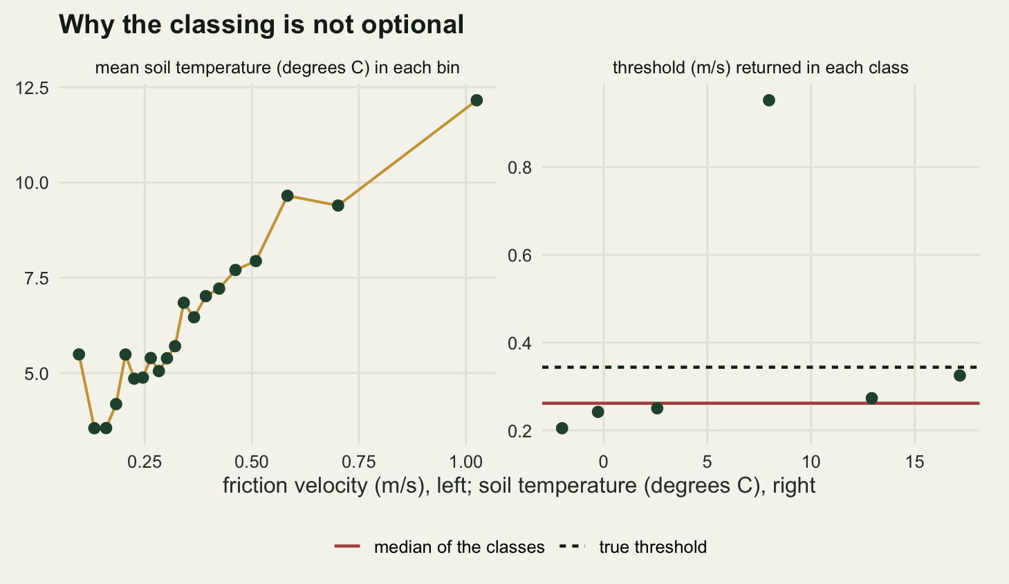
             6.0000 

The six classes return 0.205, 0.242, 0.25, 0.952, 0.273 and 0.325 m/s. One of them is absurd: the fourth class returns 0.952, which is above almost every night-time friction velocity in the record and means the rule never triggered inside that class at all. This is why the summary across classes is a median rather than a mean, and it is the single most useful piece of engineering in the whole procedure. The median comes out at 0.2617 m/s against a true 0.3438, an error of -0.0821 m/s or -23.9 per cent.

The estimate is low, and three comparisons separate the candidate reasons: what the rule would converge on with infinite clean data, what it returns on the attenuated flux with the noise switched off, and what it returns on the true unattenuated flux.

u_grid <- seq(0.05, 0.7, by = 0.001)
plateau <- vapply(u_grid, function(x) mean(att[is_night][nu > x]), numeric(1))
u_target <- u_grid[which(plogis((u_grid - u_mid) / u_w) >= 0.99 * plateau)[1]]

u_clean <- mpt_classed(nu, nee_att[is_night], nt)$med
u_notrb <- mpt_classed(nu, nee_true[is_night], nt)$med

print(round(c(true_threshold = u_true,
              population_target_of_rule = u_target,
              rule_on_noise_free_attenuated = u_clean,
              rule_on_noisy_attenuated = u_hat,
              rule_on_unattenuated_flux = u_notrb), 4))

               true_threshold     population_target_of_rule 
                       0.3438                        0.3370 
rule_on_noise_free_attenuated      rule_on_noisy_attenuated 
                       0.3522                        0.2617 
    rule_on_unattenuated_flux 
                       0.1352 

print(round(c(criterion_effect = u_target - u_true,
              binning_effect = u_clean - u_target,
              noise_effect = u_hat - u_clean), 4))

criterion_effect   binning_effect     noise_effect 
         -0.0068           0.0152          -0.0905 

The rule’s own target is not the true threshold. Because the ninety-nine per cent criterion is measured against the mean of the higher bins, and those bins are themselves attenuated by a hair, the value the rule converges on is 0.337 m/s rather than 0.3438, an offset of -0.0068. Applied to the attenuated flux with no measurement noise the classed rule returns 0.3522, which overshoots that target by 0.0152 and is close enough to the truth to be called correct.

The noise is what breaks it. Adding the measurement error moves the estimate from 0.3522 to 0.2617, a shift of -0.0905 m/s, which is the whole of the error. The mechanism is in the shape of the rule: it takes the first bin that crosses the criterion, so a bin whose mean is pushed up by chance stops the walk early, twenty bins each get a chance to end the search, and the search only ever ends too soon. A first-crossing rule is biased downwards by noise, and more data does not fix it, because sharper bin means do not remove the asymmetry. That is one of the arguments Barr et al (2013) make for replacing the walk with a fitted change point, which uses all the bins at once. Run the same classed rule on the true unattenuated flux, where there is no threshold to find, and it returns 0.1352 m/s: not zero, since the temperature classes are wide enough for some residual gradient to survive inside them, but low enough that the procedure is not inventing thresholds out of nothing.

What the temperature classing buys

Skipping the classing is the obvious simplification, and it is a disaster here. Running the same walk on the pooled night-time record gives an answer, and the answer is meaningless.

u_pool <- mpt_bin(nu, nf)
u_pool_true <- mpt_bin(nu, nee_true[is_night])
cor_all <- cor(nu, nt)

print(round(c(pooled_estimate = u_pool,
              classed_estimate = u_hat,
              true_threshold = u_true,
              pooled_bias = u_pool - u_true,
              pooled_over_classed = u_pool / u_hat), 4))

    pooled_estimate    classed_estimate      true_threshold         pooled_bias 
             1.0253              0.2617              0.3438              0.6815 
pooled_over_classed 
             3.9184 

print(round(c(cor_ustar_soil_all_night = cor_all,
              max_abs_within_class = max(abs(cc$rho)),
              mean_abs_within_class = mean(abs(cc$rho)),
              night_data_above_pooled = mean(nu >= u_pool)), 4))

cor_ustar_soil_all_night     max_abs_within_class    mean_abs_within_class 
                  0.2781                   0.3244                   0.1587 
 night_data_above_pooled 
                  0.0169 

print(round(c(pooled_on_unattenuated = u_pool_true,
              top_bin_ustar = pool_tab$ustar[20]), 4))

pooled_on_unattenuated          top_bin_ustar 
                1.0253                 1.0253 

The pooled walk returns 1.0253 m/s, which is not an overestimate of the threshold but the rule failing to trigger at all and falling out of the loop at the top bin, hence a value equal to that bin’s mean friction velocity of 1.0253. Applying it would keep 1.69 per cent of the night-time record. Run it on the true unattenuated flux and it returns 1.0253 as well: the pooled curve gives the same answer when there is nothing to find.

The correlation between friction velocity and soil temperature across all night-time half hours is 0.278. Inside the six temperature classes the largest absolute correlation is 0.324 and the average 0.159, all below the limit of 0.4 that Papale et al (2006) set for discarding a class. The classing has not abolished the confounding; it has cut it to a size the rule can survive. A correlation of 0.278 sounds mild, and the reason something that mild does so much damage is the size of the criterion: the rule is testing for a one per cent difference in mean flux, while the temperature gradient across the pooled bins is 8.61 degrees C, worth tens of per cent at this respiration sensitivity. A confounder does not have to be strong. It only has to be stronger than one per cent.

Figure 3: Left: mean soil temperature in each of the twenty pooled friction velocity bins, showing that the bins differ by several degrees and therefore in expected respiration. Right: the threshold returned inside each of the six soil temperature classes, against the mean temperature of the class, with the median across classes and the true threshold marked. The fourth class returns a value off the top of the sensible range, which is what the median is there to absorb.

What the filter costs in data

Two fractions are worth reporting and they are routinely confused. The filter removes night-time half hours only, so its effect on the night-time record is roughly twice its effect on the record as a whole.

gapi <- is_night & ustar < u_hat
keep_n <- is_night & !gapi
frac_all <- mean(gapi)
frac_night <- mean(nu < u_hat)
frac_at_true <- mean(nu < u_true)
run_len <- rle(gapi)
long_runs <- run_len$lengths[run_len$values]

print(round(c(discarded_half_hours = sum(gapi),
              fraction_of_all = frac_all,
              fraction_of_night = frac_night,
              fraction_of_night_at_true_threshold = frac_at_true,
              nights_wholly_lost = sum(tapply(gapi[is_night], nid, all))), 4))

               discarded_half_hours                     fraction_of_all 
                          3239.0000                              0.1849 
                  fraction_of_night fraction_of_night_at_true_threshold 
                             0.3697                              0.5811 
                 nights_wholly_lost 
                            40.0000 

print(round(c(gap_runs = length(long_runs),
              median_run_half_hours = median(long_runs),
              longest_run_half_hours = max(long_runs),
              mean_true_flux_discarded = mean(nee_true[gapi]),
              mean_true_flux_retained = mean(nee_true[keep_n])), 4))

                gap_runs    median_run_half_hours   longest_run_half_hours 
                412.0000                   4.0000                  32.0000 
mean_true_flux_discarded  mean_true_flux_retained 
                  1.4480                   2.0334 

At the estimated threshold the filter throws away 3239 half hours, which is 18.49 per cent of the year and 36.97 per cent of the night-time record. Had it been set at the true threshold it would have taken 58.11 per cent of the nights instead, so the estimator’s downward error is also, quietly, a decision to keep an extra 21.13 per cent of night-time data that should have gone.

The gaps are not scattered. They come in 412 runs with a median length of 4 half hours and a longest run of 32, and 40 nights lose every one of their half hours: a gap of one half hour can be interpolated, a whole week of calm November nights cannot. The true flux on the discarded half hours averages 1.448 umol/m2/s and on the retained ones 2.033, so what the filter removes is not a random sample of the night but systematically the colder, quieter part of it, with genuinely lower respiration. Any method that fills those gaps with an average of the surviving data will put back too much carbon.

The annual number

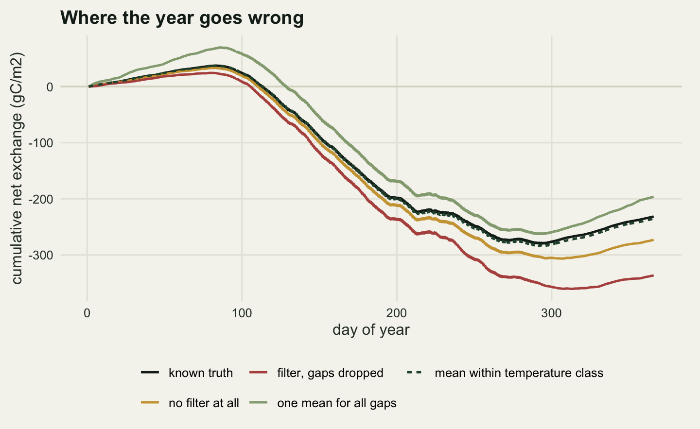
Now the sum. Five versions, all of the same year.

c_nofilt <- sum(nee_obs) * conv
c_drop <- sum(nee_obs[!gapi]) * conv
imp_flat <- mean(nee_obs[keep_n])
c_flat <- (sum(nee_obs[!gapi]) + sum(gapi) * imp_flat) * conv

br_t <- quantile(tsoil[is_night], seq(0, 1, length.out = 11))
br_t[1] <- -Inf
br_t[length(br_t)] <- Inf
cl_t <- cut(tsoil, br_t, labels = FALSE)
annual_cls <- function(thr, obs = nee_obs) {
  gi <- is_night & ustar < thr
  nk <- is_night & !gi
  mm <- as.numeric(tapply(obs[nk], factor(cl_t[nk], levels = seq_len(10)), mean))
  if (anyNA(mm)) mm[is.na(mm)] <- mean(obs[nk])
  (sum(obs[!gi]) + sum(mm[cl_t[gi]])) * conv
}
c_cls <- annual_cls(u_hat)

budget <- data.frame(
  method = c("known truth", "no filter at all", "filter, gaps dropped",
             "filter, one mean for all gaps", "filter, mean within temperature class"),
  gC = c(c_true, c_nofilt, c_drop, c_flat, c_cls))
budget$error <- budget$gC - c_true
print(round(budget[, c("gC", "error")], 2))

       gC   error
1 -231.46    0.00
2 -273.08  -41.61
3 -336.37 -104.91
4 -196.46   35.00
5 -235.38   -3.92

print(budget$method)

[1] "known truth"                          
[2] "no filter at all"                     
[3] "filter, gaps dropped"                 
[4] "filter, one mean for all gaps"        
[5] "filter, mean within temperature class"

print(round(c(imputed_value = imp_flat,
              true_mean_on_gaps = mean(nee_true[gapi]),
              over_imputation = imp_flat - mean(nee_true[gapi])), 4))

    imputed_value true_mean_on_gaps   over_imputation 
           1.9979            1.4480            0.5499 

Against a true -231.46 gC/m2/yr, the unfiltered sum comes out at -273.08, overstating the sink by 41.61 gC/m2/yr or 18 per cent. That is the attenuation arriving in the answer: carbon that left the fen but was never measured leaving it.

Filtering and then dropping the discarded half hours from the sum gives -336.37, which is worse than doing nothing at all by a wide margin, for a reason that is arithmetic rather than ecological. A sum over a subset is not an estimate of the sum over the whole; dropping a value from a total is imputing zero for it, and the values being dropped are all positive night-time releases. The filter identified the bad half hours correctly and then the sum threw away the carbon along with them.

Replacing each gap with the mean of the retained night-time data gives -196.46, an error of 35 gC/m2/yr in the other direction. This is the honest name for what dropping was trying to be: mean imputation. It is better than zero imputation by a factor of 3, and it is still wrong, for the reason the previous section flagged. The imputed value is 1.998 umol/m2/s while the true mean on the gaps is 1.448, an over-imputation of 0.55 umol/m2/s on every one of 3239 half hours.

The last row is the crudest possible improvement: sort the retained night-time data into ten soil temperature classes and fill each gap with the mean of its own class. That gives -235.38, an error of -3.92 gC/m2/yr, so a single covariate used in the bluntest possible way removes almost the whole of the imputation error. There is no comparison of filling methods here, and that is the next post’s job; the point is that the residual error after filtering is an imputation problem rather than a filtering problem, and that the choice of fill changes the annual number by more than the filter does.

Figure 4: Cumulative net ecosystem exchange through the year under four treatments of the same measurements, against the known truth. Dropping the filtered half hours from the sum pulls steadily away from the truth all year, because every discarded value is a positive night-time release replaced by nothing. Filling every gap with one mean over-corrects. Filling within soil temperature classes tracks the truth.

How well is the threshold known

The threshold is a statistic and it has a sampling distribution. The resampling unit has to be the night, not the half hour: half hours inside one night share a weather state, a temperature and a turbulence regime, and resampling them individually would treat a year as if it held seventeen thousand independent observations of turbulence rather than a few hundred. Papale et al (2006) resample this way, and report that of all the processing choices in a flux chain the friction velocity correction contributes most to the uncertainty of an annual figure.

set.seed(20260805)
nights <- unique(nid)
n_night <- length(nights)
by_night <- split(seq_along(nid), nid)
n_boot <- 300
boot_u <- numeric(n_boot)
for (b in seq_len(n_boot)) {
  pick <- unlist(by_night[as.character(sample(nights, n_night, replace = TRUE))],
                 use.names = FALSE)
  boot_u[b] <- mpt_classed(nu[pick], nf[pick], nt[pick])$med
}

annual_flat <- function(thr, obs = nee_obs) {
  gi <- is_night & ustar < thr
  nk <- is_night & !gi
  (sum(obs[!gi]) + sum(gi) * mean(obs[nk])) * conv
}
boot_flat <- vapply(boot_u, annual_flat, numeric(1))
boot_cls <- vapply(boot_u, annual_cls, numeric(1))

print(round(c(replicates = n_boot, nights_resampled = n_night,
              point_estimate = u_hat, boot_mean = mean(boot_u),
              boot_sd = sd(boot_u),
              boot_q05 = unname(quantile(boot_u, 0.05)),
              boot_q95 = unname(quantile(boot_u, 0.95)),
              true_threshold = u_true), 4))

      replicates nights_resampled   point_estimate        boot_mean 
        300.0000         366.0000           0.2617           0.2776 
         boot_sd         boot_q05         boot_q95   true_threshold 
          0.0199           0.2463           0.3076           0.3438 

print(round(c(flat_sd = sd(boot_flat), flat_q05 = unname(quantile(boot_flat, 0.05)),
              flat_q95 = unname(quantile(boot_flat, 0.95)),
              class_sd = sd(boot_cls), class_q05 = unname(quantile(boot_cls, 0.05)),
              class_q95 = unname(quantile(boot_cls, 0.95))), 3))

  flat_sd  flat_q05  flat_q95  class_sd class_q05 class_q95 
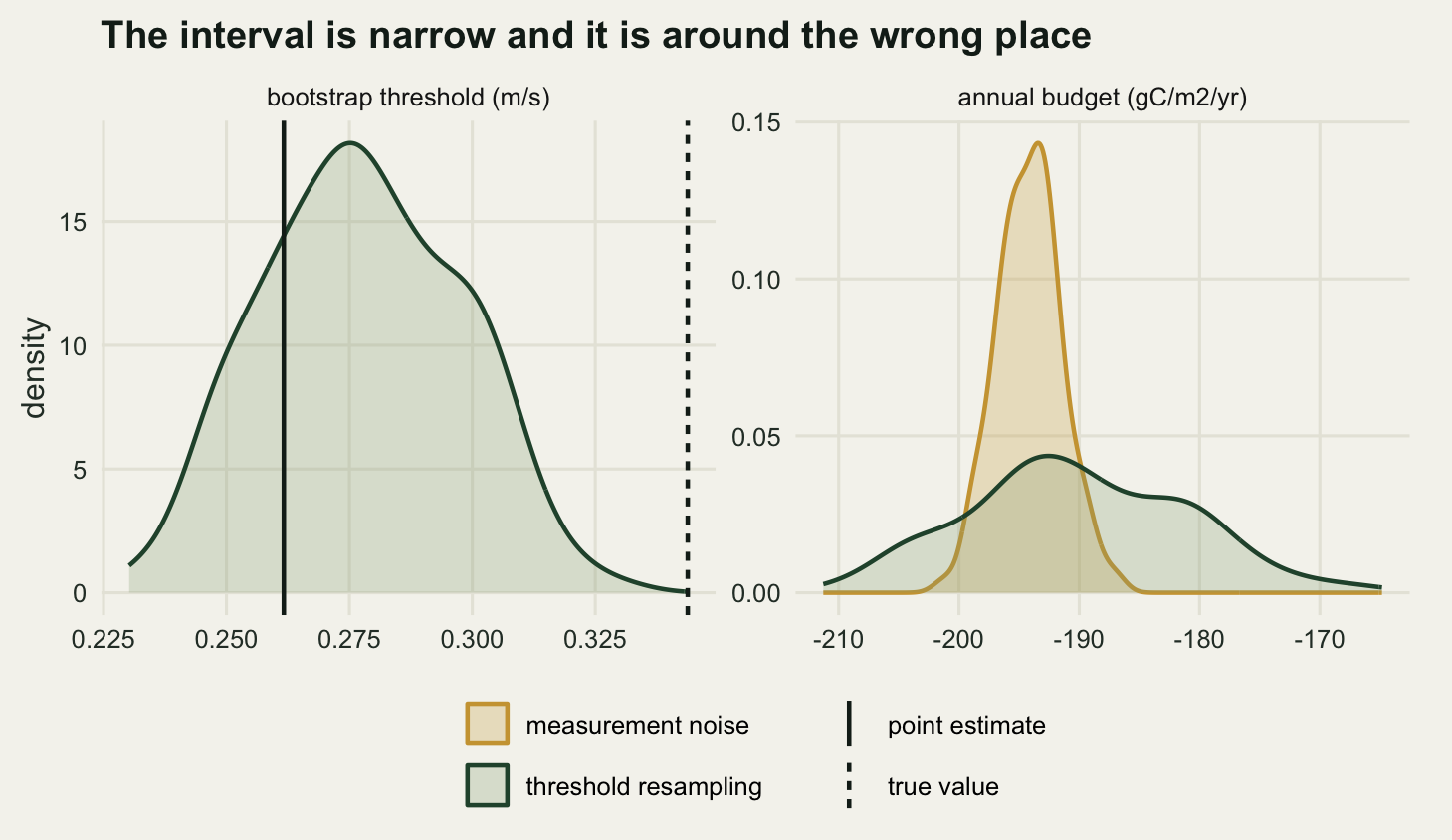
    9.045  -204.782  -176.314     1.537  -237.267  -232.328 

Over 300 resamples of the 366 nights the threshold has a standard deviation of 0.0199 m/s and a fifth to ninety-fifth percentile range of 0.2463 to 0.3076. The true value, 0.3438, lies above the ninety-fifth percentile. That is the first thing to say about the bootstrap: it is a sampling interval around a biased point estimate, and it does not contain the answer.

Pushing each of those 300 thresholds through the annual sum gives a standard deviation of 9.04 gC/m2/yr with the flat imputation and 1.54 with the temperature-class imputation. The threshold’s contribution to the budget’s uncertainty is not a property of the threshold. It is a property of the threshold and the gap filling together, and it differs between the two by a factor of 5.9.

Which matters more to the annual figure, the threshold or the random measurement noise? Both are measurable here: redraw the noise on a fixed threshold, and compare the spread of the annual sum with the spread the bootstrap produced.

set.seed(20260806)
n_noise <- 200
noise_flat <- numeric(n_noise)
noise_cls <- numeric(n_noise)
for (b in seq_len(n_noise)) {
  obs_b <- nee_att + rnorm(n_half, 0, sig)
  noise_flat[b] <- annual_flat(u_hat, obs_b)
  noise_cls[b] <- annual_cls(u_hat, obs_b)
}

set.seed(20260807)
n_both <- 150
both_flat <- numeric(n_both)
both_u <- numeric(n_both)
for (b in seq_len(n_both)) {
  obs_b <- nee_att + rnorm(n_half, 0, sig)
  both_u[b] <- mpt_classed(nu, obs_b[is_night], nt)$med
  both_flat[b] <- annual_flat(both_u[b], obs_b)
}

sys_gap <- annual_flat(u_hat) - annual_flat(u_true)
print(round(c(noise_only_flat = sd(noise_flat), noise_only_class = sd(noise_cls),
              threshold_only_flat = sd(boot_flat),
              threshold_only_class = sd(boot_cls)), 3))

     noise_only_flat     noise_only_class  threshold_only_flat 
               2.653                2.600                9.045 
threshold_only_class 
               1.537 

print(round(c(ratio_flat = sd(boot_flat) / sd(noise_flat),
              ratio_class = sd(boot_cls) / sd(noise_cls),
              noise_through_threshold = sd(both_flat),
              threshold_sd_from_noise = sd(both_u)), 4))

             ratio_flat             ratio_class noise_through_threshold 
                 3.4088                  0.5910                  9.2540 
threshold_sd_from_noise 
                 0.0171 

print(round(c(annual_at_estimate = annual_flat(u_hat),
              annual_at_truth = annual_flat(u_true),
              systematic_gap = sys_gap,
              gap_over_boot_sd = abs(sys_gap) / sd(boot_flat)), 3))

annual_at_estimate    annual_at_truth     systematic_gap   gap_over_boot_sd 
          -196.462           -161.736            -34.727              3.839 

Under the flat imputation it is the threshold, by a clear margin: a standard deviation of 9.04 gC/m2/yr against 2.65 from the measurement noise, a ratio of 3.41. Under the temperature-class imputation it is the noise: 1.54 against 2.6, a ratio of 0.59. The familiar claim that the threshold dominates the random error is true of this simulation under a crude gap fill and false under a slightly less crude one, so stating it without saying which gap fill is meant says nothing.

Two further numbers matter more than the ratio. Redrawing the noise and re-estimating the threshold from the redrawn data gives a spread of 9.25 gC/m2/yr, with the threshold itself varying by 0.0171 m/s across those draws. So the measurement noise is not a separate small term to be added to the threshold uncertainty: a large part of the threshold uncertainty is measurement noise, arriving through the estimator rather than through the sum.

And the systematic error dwarfs both. Evaluating the annual sum at the estimated threshold gives -196.46 gC/m2/yr and at the true threshold -161.74, a gap of -34.73 gC/m2/yr, which is 3.8 times the bootstrap standard deviation. A published uncertainty built from resampling alone would quote a range that excludes the value the correct threshold produces. Note also which of the two is closer to the truth: the biased threshold, at -196.46 against a true -231.46, beats the correct one at -161.74, because a filter that discards more data gives the biased imputation more to be wrong about. Two errors partly cancelling is not a method.

Figure 5: Left: the distribution of the friction velocity threshold over three hundred bootstrap resamples of whole nights, with the point estimate and the true threshold marked. The true value sits outside the bulk of the distribution. Right: the annual budget’s spread from threshold resampling and from redrawing the measurement noise, under the flat gap fill. The threshold distribution is much the wider of the two.

The honest limit

Everything above rests on one property of the simulation that no tower has: the attenuation is a known function of a single variable. Friction velocity was the only thing that decided how much flux got through, so a filter on friction velocity could in principle be exactly right, and the only question was whether the estimator found the number.

A real calm night is not like that. The carbon that fails to reach the sensor has at least three destinations and the filter addresses one of them. Some is stored in the canopy air below the instrument and released in a burst at sunrise, which a storage term from a concentration profile can partly recover and which single-point storage estimates handle badly. Some drains downslope as a density current, and on anything other than flat ground that advective loss is not a function of friction velocity at all: Aubinet (2008) reviews the nocturnal problem and concludes that the advective term cannot be reliably measured with the instrumentation most towers carry. Massman and Lee (2002) set the friction velocity filter alongside the other corrections a flux record needs and note that they interact rather than adding up independently. Some of it simply goes missing.

The seasonality in this simulation is a second limit and it was put there deliberately. Friction velocity was made to depend on canopy greenness, so the same wind gives a higher friction velocity in July than in February. A threshold estimated over the whole year is therefore a compromise between two different canopies, and the temperature classing that rescues the estimate is doing double duty, separating both the respiration response and the roughness change. On a real site the canopy changes, the fetch changes with wind direction, and instruments are cleaned and replaced. A threshold estimated in one season is not guaranteed to hold in another, which is why some implementations estimate the threshold season by season and then take the largest of the seasonal values. That is a different convention, it will in general return a different number, and neither version is checkable.

The third limit is the one that makes the other two permanent. There is no truth column at a flux tower. The annual figure of -231.46 gC/m2/yr that every method here was scored against exists only because the data were generated. In the field the threshold is chosen by a convention: ninety-nine per cent of the plateau, six temperature classes, twenty bins, the median across classes, resample the nights. Change any one of those and the number changes, and there is nothing in the data to say which choice was right. The convention is what makes annual budgets from different towers comparable with each other, and that is a real and sufficient reason to follow it, but comparability is not accuracy.

Where to go next

The record this post leaves behind has 3239 holes in it, they arrive in runs of up to 32 half hours, and they are not missing at random: they are the coldest and quietest part of every night. Filling them is gap filling a flux time series, and the last two sections here are the argument for why that post exists, since the choice of fill changed the annual number by more than the filter did. Once the record is complete, splitting it into gross uptake and respiration is partitioning net flux into GPP and respiration, which fits the same Lloyd and Taylor curve used to generate the data here, to night-time data that has been through this filter. The audit of the finished annual figure, including how much of its uncertainty traces back to the threshold, is checking an annual flux budget.

For the wider machinery: resampling whole nights rather than half hours is the idea behind bootstrapping dependent data: blocks and clusters, and the general treatment of resampled intervals is bootstrap confidence intervals. The non-random hole this filter cuts is a missing-not-at-random problem, whose general form is missing data: MCAR, MAR and MNAR. The litter cluster, doing the same carbon accounting with a balance instead of a sonic anemometer, starts at fitting litter decomposition curves.

References

Goulden ML, Munger JW, Fan SM, Daube BC, Wofsy SC 1996 Global Change Biology 2(3):169-182 (10.1111/j.1365-2486.1996.tb00070.x)

Aubinet M, Grelle A, Ibrom A, Rannik U, Moncrieff J, Foken T, Kowalski AS, Martin PH, Berbigier P, Bernhofer C, Clement R, Elbers J, Granier A, Grunwald T, Morgenstern K, Pilegaard K, Rebmann C, Snijders W, Valentini R, Vesala T 2000 Advances in Ecological Research 30:113-175 (10.1016/S0065-2504(08)60018-5)

Massman WJ, Lee X 2002 Agricultural and Forest Meteorology 113(1-4):121-144 (10.1016/S0168-1923(02)00105-3)

Gu L, Falge EM, Boden T, Baldocchi DD, Black TA, Saleska SR, Suni T, Verma SB, Vesala T, Wofsy SC, Xu L 2005 Agricultural and Forest Meteorology 128(3-4):179-197 (10.1016/j.agrformet.2004.11.006)

Papale D, Reichstein M, Aubinet M, Canfora E, Bernhofer C, Kutsch W, Longdoz B, Rambal S, Valentini R, Vesala T, Yakir D 2006 Biogeosciences 3(4):571-583 (10.5194/bg-3-571-2006)

Richardson AD, Hollinger DY, Burba GG, Davis KJ, Flanagan LB, Katul GG, Munger JW, Ricciuto DM, Stoy PC, Suyker AE, Verma SB, Wofsy SC 2006 Agricultural and Forest Meteorology 136(1-2):1-18 (10.1016/j.agrformet.2006.01.007)

Aubinet M 2008 Ecological Applications 18(6):1368-1378 (10.1890/06-1336.1)

Barr AG, Richardson AD, Hollinger DY, Papale D, Arain MA, Black TA, Bohrer G, Dragoni D, Fischer ML, Gu L, Law BE, Margolis HA, McCaughey JH, Munger JW, Oechel W, Schaeffer K 2013 Agricultural and Forest Meteorology 171-172:31-45 (10.1016/j.agrformet.2012.11.023)

Lloyd J, Taylor JA 1994 Functional Ecology 8(3):315-323 (10.2307/2389824)

Related tutorials

• Gap filling a flux time series
• Partitioning net flux into GPP and respiration
• Checking an annual flux budget
• Mass loss and the carbon budget