---
title: "Missing data: MCAR, MAR and MNAR"
description: "The three missing-data mechanisms in R: why complete-case deletion stays unbiased under MCAR, shifts the mean under MAR, and biases the slope too under MNAR."
date: "2026-05-28 10:00"
categories: [R, missing data, ggplot2, ecology tutorial]
image: thumbnail.png
image-alt: "Two panels of complete-case sampling distributions showing the mean biased under MAR and MNAR but the slope biased only under MNAR."
---
Gaps are the rule, not the exception, in ecological data: a logger fails, an animal is never recaptured, a covariate is recorded for some sites and not others. The reflex is to drop every row with a gap and analyse what is left, the complete-case (or listwise) analysis. Whether that is safe depends entirely on *why* the values are missing, and on *what* you are trying to estimate. This post sets out the three mechanisms behind missing data and shows, by simulation, that the same deletion is harmless in one setting and badly misleading in another.
The running example is a simple linear relationship between a predictor `x` (always recorded) and a response `y` (sometimes missing), with two targets of interest: the mean of `y`, and the slope of `y` on `x`.
```{r}
#| label: setup
#| message: false
#| warning: false
#| code-fold: true
#| code-summary: "Setup: packages, colours and plot theme"
library(ggplot2); library(dplyr); library(tidyr)
ink <- "#2b2b2b"; grid_col <- "#d9d5cc"; paper <- "#f5f4ee"
col_full <- "#6f6f6f"; col_obs <- "#356170"
pal <- c(MCAR = "#4a7a8c", MAR = "#c08a3e", MNAR = "#a24b4b")
theme_te <- function(base = 12) {
  theme_minimal(base_size = base) +
    theme(panel.grid.minor = element_blank(),
          panel.grid.major = element_line(colour = grid_col, linewidth = 0.3),
          plot.background = element_rect(fill = paper, colour = NA),
          panel.background = element_rect(fill = paper, colour = NA),
          strip.text = element_text(face = "bold", colour = ink),
          plot.title = element_text(face = "bold", colour = ink),
          axis.title = element_text(colour = ink),
          legend.position = "top")
}
```
## The three mechanisms
Rubin (1976) split the reasons a value can be absent into three cases, defined by what the probability of being missing depends on.
*Missing completely at random* (MCAR): the chance of a gap is unrelated to anything, observed or not. A logger battery that fails on a random schedule is MCAR. The recorded values are a plain random subset of the full data.
*Missing at random* (MAR): the chance of a gap depends only on values you *do* observe. If sites with high `x` are harder to revisit, so their `y` is more often missing, the missingness depends on the observed `x`, not on the unseen `y` itself. The name is unfortunate: MAR does not mean the gaps are random, it means they are random once you condition on the observed data.
*Missing not at random* (MNAR): the chance of a gap depends on the missing value itself, even after accounting for what you observe. If large individuals are the ones that slip the net, so their body size is missing *because* it is large, the value drives its own absence.
The three cannot be told apart from the recorded values alone, a point we return to at the end. Here we know the mechanism because we impose it.
```{r}
#| label: dgp
set.seed(6813)
n <- 600; b0 <- 5; b1 <- 2; sde <- 2
x <- rnorm(n, 0, 1)
y <- b0 + b1 * x + rnorm(n, 0, sde)
full_mean  <- mean(y)
full_slope <- unname(coef(lm(y ~ x))[2])

## impose each mechanism on y, targeting about 40% missing
p_mcar <- rep(0.40, n)                                   # unrelated to anything
a1 <- 1.2                                                # MAR: depends on observed x
a0 <- uniroot(function(a) mean(plogis(a + a1 * x)) - 0.40, c(-5, 5))$root
p_mar <- plogis(a0 + a1 * x)
ys <- as.numeric(scale(y)); g1 <- 1.2                    # MNAR: depends on y itself
g0 <- uniroot(function(g) mean(plogis(g + g1 * ys)) - 0.40, c(-5, 5))$root
p_mnar <- plogis(g0 + g1 * ys)

blank <- function(p) { yo <- y; yo[runif(n) < p] <- NA; yo }
yo_mcar <- blank(p_mcar); yo_mar <- blank(p_mar); yo_mnar <- blank(p_mnar)

cc_mean  <- function(yo) mean(yo, na.rm = TRUE)
cc_slope <- function(yo) { ok <- !is.na(yo); unname(coef(lm(yo[ok] ~ x[ok]))[2]) }
```
The full data give a mean of `r round(full_mean, 3)` (truth 5) and a slope of `r round(full_slope, 3)` (truth 2). Each mechanism blanks out roughly `r round(100 * mean(is.na(yo_mar)))`% of the responses.
## Complete-case deletion, mechanism by mechanism
Delete the blanked rows and re-estimate. The mean of `y` first:
```{r}
#| label: cc-mean
round(c(full = full_mean,
        MCAR = cc_mean(yo_mcar),
        MAR  = cc_mean(yo_mar),
        MNAR = cc_mean(yo_mnar)), 3)
```
Under MCAR the complete-case mean is `r round(cc_mean(yo_mcar), 3)`, against the full-data `r round(full_mean, 3)`. Under MAR it falls to `r round(cc_mean(yo_mar), 3)` and under MNAR to `r round(cc_mean(yo_mnar), 3)`. Both are pulled below the truth of 5, because dropping the high-`x` (and so high-`y`) sites under MAR, or the high-`y` sites directly under MNAR, throws away the top of the response distribution.
Now the slope of `y` on `x`, the same deletions:
```{r}
#| label: cc-slope
round(c(full = full_slope,
        MCAR = cc_slope(yo_mcar),
        MAR  = cc_slope(yo_mar),
        MNAR = cc_slope(yo_mnar)), 3)
```
Here the picture changes. The MCAR slope is `r round(cc_slope(yo_mcar), 3)`, the MAR slope is `r round(cc_slope(yo_mar), 3)` and the MNAR slope is `r round(cc_slope(yo_mnar), 3)`, against a true 2.
The regression already conditions on `x`. When missingness depends only on `x`, it is unrelated to `y` *within* each value of `x`, so the conditional relationship of `y` given `x` survives deletion untouched. The marginal mean does not, because selecting on `x` selects on the correlated `y`. Under MNAR the gaps depend on `y` given `x`, which truncates the response at each `x` and bends the line.
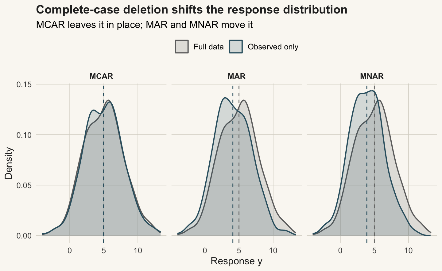
Figure 1 makes the mean shift visible: under MCAR the observed density sits on top of the full one, while MAR and MNAR pull it left.
```{r}
#| label: fig-densities
#| fig-cap: "Full-data response distribution against the observed-only distribution after complete-case deletion, for each mechanism. Dashed lines mark the group means."
#| fig-alt: "Three density panels for MCAR, MAR and MNAR. Under MCAR the observed and full densities overlap; under MAR and MNAR the observed density and its mean shift to the left of the full data."
#| fig-width: 7.5
#| fig-height: 4.6
mk <- function(yo, nm) rbind(
  data.frame(y = y, set = "Full data", mech = nm),
  data.frame(y = yo[!is.na(yo)], set = "Observed only", mech = nm))
df1 <- rbind(mk(yo_mcar, "MCAR"), mk(yo_mar, "MAR"), mk(yo_mnar, "MNAR"))
df1$mech <- factor(df1$mech, levels = c("MCAR", "MAR", "MNAR"))
mu1 <- df1 |> group_by(mech, set) |> summarise(m = mean(y), .groups = "drop")
ggplot(df1, aes(y, colour = set, fill = set)) +
  geom_density(alpha = 0.18, linewidth = 0.7) +
  geom_vline(data = mu1, aes(xintercept = m, colour = set),
             linetype = "dashed", linewidth = 0.5, show.legend = FALSE) +
  facet_wrap(~mech) +
  scale_colour_manual(values = c("Full data" = col_full, "Observed only" = col_obs)) +
  scale_fill_manual(values = c("Full data" = col_full, "Observed only" = col_obs)) +
  labs(title = "Complete-case deletion shifts the response distribution",
       subtitle = "MCAR leaves it in place; MAR and MNAR move it",
       x = "Response y", y = "Density", colour = NULL, fill = NULL) +
  theme_te()
```
## Bias and coverage across many datasets
One dataset can mislead, so repeat the whole exercise 2000 times, recording the complete-case estimate and whether its 95% Wald interval covers the truth.
```{r}
#| label: monte-carlo
M <- 2000
res <- matrix(NA, M, 6,
  dimnames = list(NULL, c("mean_MCAR", "mean_MAR", "mean_MNAR",
                          "slope_MCAR", "slope_MAR", "slope_MNAR")))
cov <- res
set.seed(20240613)
for (i in 1:M) {
  xx <- rnorm(n, 0, 1); yy <- b0 + b1 * xx + rnorm(n, 0, sde)
  yys <- as.numeric(scale(yy))
  a0i <- uniroot(function(a) mean(plogis(a + a1 * xx)) - 0.40, c(-6, 6))$root
  g0i <- uniroot(function(g) mean(plogis(g + g1 * yys)) - 0.40, c(-6, 6))$root
  ms <- list(MCAR = runif(n) < 0.40,
             MAR  = runif(n) < plogis(a0i + a1 * xx),
             MNAR = runif(n) < plogis(g0i + g1 * yys))
  for (j in seq_along(ms)) {
    yo <- yy; yo[ms[[j]]] <- NA; ok <- !is.na(yo)
    mu <- mean(yo, na.rm = TRUE); se_mu <- sd(yo, na.rm = TRUE) / sqrt(sum(ok))
    res[i, j] <- mu
    cov[i, j] <- (mu - 1.96 * se_mu <= b0) & (b0 <= mu + 1.96 * se_mu)
    fit <- lm(yo[ok] ~ xx[ok]); bs <- unname(coef(fit)[2]); se_b <- summary(fit)$coef[2, 2]
    res[i, j + 3] <- bs
    cov[i, j + 3] <- (bs - 1.96 * se_b <= b1) & (b1 <= bs + 1.96 * se_b)
  }
}
mc <- rbind(bias = colMeans(res) - rep(c(b0, b1), each = 3),
            coverage = colMeans(cov))
round(mc, 3)
```
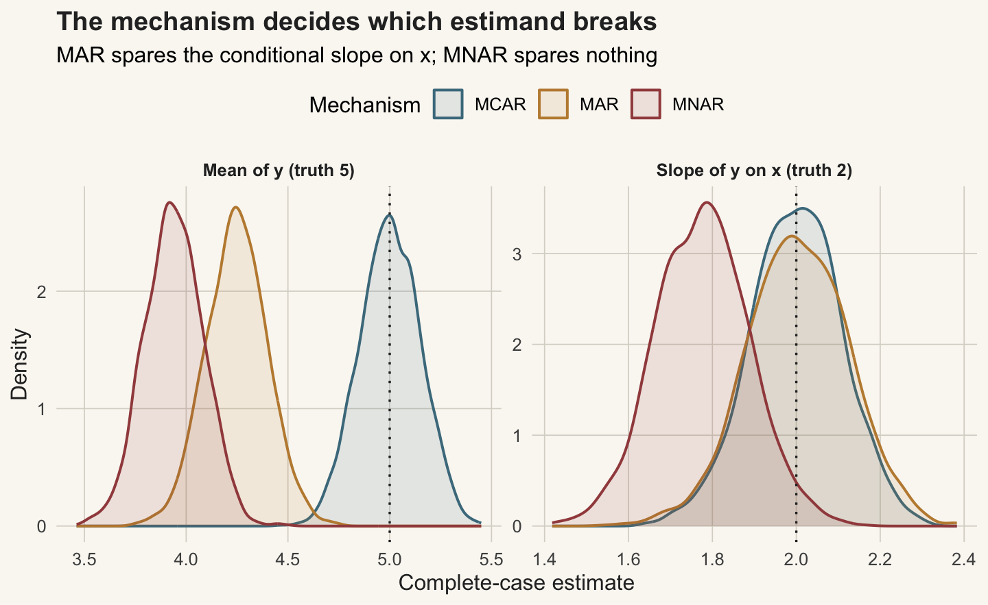
The mean is unbiased only under MCAR (bias `r sprintf("%.3f", mc["bias","mean_MCAR"])`, coverage `r round(100*mc["coverage","mean_MCAR"])`%); under MAR its bias is `r sprintf("%.2f", mc["bias","mean_MAR"])` and coverage collapses to `r round(100*mc["coverage","mean_MAR"], 1)`%, under MNAR worse still. The slope is unbiased under both MCAR *and* MAR (coverage `r round(100*mc["coverage","slope_MCAR"])`% and `r round(100*mc["coverage","slope_MAR"])`%), and only MNAR breaks it (bias `r sprintf("%.3f", mc["bias","slope_MNAR"])`, coverage `r round(100*mc["coverage","slope_MNAR"], 1)`%). Figure 2 shows the two estimands side by side.
```{r}
#| label: fig-sampling
#| fig-cap: "Sampling distributions of the complete-case mean and slope over 2000 datasets, by mechanism. Dotted lines mark the truth. MAR biases the mean but not the slope on x; MNAR biases both."
#| fig-alt: "Two density panels. The left panel, mean of y, shows MAR and MNAR shifted left of the truth while MCAR is centred on it. The right panel, slope on x, shows MCAR and MAR centred on the truth and only MNAR shifted."
#| fig-width: 7.5
#| fig-height: 4.6
rd <- as.data.frame(res)
df2 <- rbind(
  data.frame(est = rd$mean_MCAR,  mech = "MCAR", target = "Mean of y (truth 5)"),
  data.frame(est = rd$mean_MAR,   mech = "MAR",  target = "Mean of y (truth 5)"),
  data.frame(est = rd$mean_MNAR,  mech = "MNAR", target = "Mean of y (truth 5)"),
  data.frame(est = rd$slope_MCAR, mech = "MCAR", target = "Slope of y on x (truth 2)"),
  data.frame(est = rd$slope_MAR,  mech = "MAR",  target = "Slope of y on x (truth 2)"),
  data.frame(est = rd$slope_MNAR, mech = "MNAR", target = "Slope of y on x (truth 2)"))
df2$mech <- factor(df2$mech, levels = c("MCAR", "MAR", "MNAR"))
tru <- data.frame(target = c("Mean of y (truth 5)", "Slope of y on x (truth 2)"), v = c(5, 2))
ggplot(df2, aes(est, colour = mech, fill = mech)) +
  geom_density(alpha = 0.12, linewidth = 0.7) +
  geom_vline(data = tru, aes(xintercept = v), colour = ink, linetype = "dotted", linewidth = 0.6) +
  facet_wrap(~target, scales = "free") +
  scale_colour_manual(values = pal) + scale_fill_manual(values = pal) +
  labs(title = "The mechanism decides which estimand breaks",
       subtitle = "MAR spares the conditional slope on x; MNAR spares nothing",
       x = "Complete-case estimate", y = "Density", colour = "Mechanism", fill = "Mechanism") +
  theme_te()
```
## The honest limit
Two lessons sit underneath the simulation. First, complete-case deletion is not uniformly bad or uniformly safe: under MCAR it costs only precision, under MAR it can leave a conditional regression intact while ruining a marginal mean, and under MNAR it distorts almost everything. What breaks depends on the mechanism *and* the quantity you want. Second, and more awkward, the mechanism is not something the recorded data can reveal. A test can reject MCAR by showing that missingness is associated with observed values (the next post in this series returns to this), but no amount of observed data can separate MAR from MNAR, because the two differ only in how missingness relates to the values you never see. Choosing between them is an assumption about the process, argued from field knowledge, not read off the dataset. Every principled repair of missing data, imputation included, rests on such an assumption; the rest of this series takes MAR as the working case and then asks what happens when it is wrong.
This is a technical account of a method; if a real analysis hinges on it, treat the mechanism as a judgement to defend, not a setting to pick.
## References
Rubin DB 1976. Biometrika 63(3):581-592 (10.1093/biomet/63.3.581).
Little RJA 1988. Journal of the American Statistical Association 83(404):1198-1202 (10.1080/01621459.1988.10478722).
Nakagawa S, Freckleton RP 2008. Trends in Ecology and Evolution 23(11):592-596 (10.1016/j.tree.2008.06.014).
Little RJA, Rubin DB 2019. Statistical Analysis with Missing Data, 3rd edn. Wiley. ISBN 978-0-470-52679-8.
Enders CK 2010. Applied Missing Data Analysis. Guilford Press. ISBN 978-1-60623-639-0.
## Related tutorials
- [Single imputation: bias and variance](../single-imputation-bias-variance/)
- [Multiple imputation by chained equations](../multiple-imputation-chained-equations/)
- [Checking missing-data assumptions](../checking-missing-data-assumptions/)
- [Missing values in a predictor: why, not how many](../missing-values-in-a-predictor/)