---
title: "Checking missing-data assumptions"
description: "Probing the missing-at-random assumption in R: a logistic missingness check, an observed-versus-imputed diagnostic, and a delta shift sensitivity analysis."
date: "2026-05-28 13:00"
categories: [R, missing data, simulation, ggplot2, ecology tutorial]
image: thumbnail.png
image-alt: "A sensitivity curve of a treatment effect and its interval falling as the assumed shortfall of treatment dropouts grows, ending at a little over a quarter of its starting value. The lower limit of the interval reaches zero at the marked tipping point, while the estimate itself stays above zero throughout."
---
Every method in this series has leaned on one assumption: that the data are missing at random, so that what you observe is enough to stand in for what you do not. The awkward fact, established in the first post, is that this assumption cannot be tested against the recorded data. No diagnostic can separate missing at random from missing not at random, because the two differ only in how missingness relates to values you never see. So the honest response is not a test but a two-part discipline: check what *can* be checked, the imputation model, and then probe what cannot, the mechanism, by asking how wrong the assumption would have to be to change the answer. This closing post does both.
The example is a two-group comparison. A treatment is applied to half the sample, the outcome `y` has a true effect of 0.6, and `y` is missing at random given a covariate `x`.
```{r}
#| label: setup
#| message: false
#| warning: false
#| code-fold: true
#| code-summary: "Setup: packages, colours and plot theme"
library(ggplot2); library(dplyr); library(tidyr); library(MASS)
ink <- "#2b2b2b"; grid_col <- "#d9d5cc"; paper <- "#f5f4ee"
theme_te <- function(base = 12) {
  theme_minimal(base_size = base) +
    theme(panel.grid.minor = element_blank(),
          panel.grid.major = element_line(colour = grid_col, linewidth = 0.3),
          plot.background = element_rect(fill = paper, colour = NA),
          panel.background = element_rect(fill = paper, colour = NA),
          strip.text = element_text(face = "bold", colour = ink),
          plot.title = element_text(face = "bold", colour = ink),
          axis.title = element_text(colour = ink),
          legend.position = "top")
}
## proper Bayesian linear imputation and Rubin pooling, as built in the previous post
step <- function(target, mask, preds) {
  obs <- !mask; Xo <- cbind(1, preds[obs, , drop = FALSE]); Vo <- target[obs]
  XtXinv <- chol2inv(chol(crossprod(Xo))); bhat <- XtXinv %*% crossprod(Xo, Vo)
  dfree <- sum(obs) - ncol(Xo); s2 <- sum((Vo - Xo %*% bhat)^2) / dfree
  s2s <- s2 * dfree / rchisq(1, dfree); bstar <- bhat + t(chol(s2s * XtXinv)) %*% rnorm(ncol(Xo))
  out <- target; Xm <- cbind(1, preds[mask, , drop = FALSE])
  out[mask] <- as.numeric(Xm %*% bstar) + rnorm(sum(mask), 0, sqrt(s2s)); out
}
pool <- function(ests, ses, m, nu_com) {
  Qbar <- mean(ests); Ubar <- mean(ses^2); B <- var(ests); Tt <- Ubar + (1 + 1 / m) * B
  lambda <- (1 + 1 / m) * B / Tt; nu_old <- (m - 1) / lambda^2
  nu_obs <- (nu_com + 1) / (nu_com + 3) * nu_com * (1 - lambda)
  df <- nu_old * nu_obs / (nu_old + nu_obs); c(Q = Qbar, se = sqrt(Tt), df = df)
}
```
```{r}
#| label: dgp
set.seed(3672)
ng <- 250; g <- rep(0:1, each = ng); n <- 2 * ng
x <- rnorm(n); tau <- 0.6; beta <- 0.5
y_true <- 0 + tau * g + beta * x + rnorm(n, 0, 1)
## missing at random on x: higher x makes y more likely to be missing (about 35%)
aM <- uniroot(function(a) mean(plogis(a + x)) - 0.35, c(-6, 6))$root
my <- runif(n) < plogis(aM + x)
y <- y_true; y[my] <- NA
```
About `r round(100 * mean(my))`% of outcomes are missing, similar in both groups (`r round(100*mean(my[g==0]))`% and `r round(100*mean(my[g==1]))`%). Multiple imputation under the working assumption, imputing `y` from group and `x`, recovers the effect:
```{r}
#| label: mar-fit
m <- 40; nu_com <- n - 3
imps <- lapply(1:m, function(k) step(y, my, cbind(g, x)))
eff <- function(yc) { f <- lm(yc ~ g + x); c(coef(f)["g"], summary(f)$coef["g", 2]) }
E0 <- sapply(imps, eff)
p0 <- pool(E0[1, ], E0[2, ], m, nu_com); tcrit <- qt(0.975, p0["df"])
c(effect = unname(p0["Q"]),
  lo = unname(p0["Q"] - tcrit * p0["se"]), hi = unname(p0["Q"] + tcrit * p0["se"]))
```
The pooled effect is `r round(p0["Q"], 3)`, with a 95% interval of `r round(p0["Q"]-tcrit*p0["se"], 3)` to `r round(p0["Q"]+tcrit*p0["se"], 3)`, comfortably clear of zero. Taken at face value, the treatment works. The rest of the post asks how much that conclusion depends on the assumption.
## What the observed data can rule out
One thing the data *can* do is reject the strongest assumption, that the gaps are completely at random. If missingness is unrelated to everything observed, then a model predicting whether a value is missing from the observed variables should find nothing. Fit that model.
```{r}
#| label: mcar-check
mcar <- glm(my ~ g + x, family = binomial)
round(summary(mcar)$coefficients, 3)
```
The coefficient on `x` is large and its p-value is effectively zero, so missingness depends strongly on the observed covariate: not missing completely at random. The coefficient on group is near zero (p `r round(summary(mcar)$coef["g",4], 2)`), so the two groups drop out at similar rates. This is the formal ground for a missing-at-random analysis over a complete-case one, and it is what a test such as Little's omnibus check (Little 1988) formalises across many variables at once. What it cannot do is go further. The same observed association with `x` is exactly what missing at random and missing not at random both predict; the test rejects complete randomness and then falls silent on the distinction that actually matters.
## A diagnostic that checks the model, not the mechanism
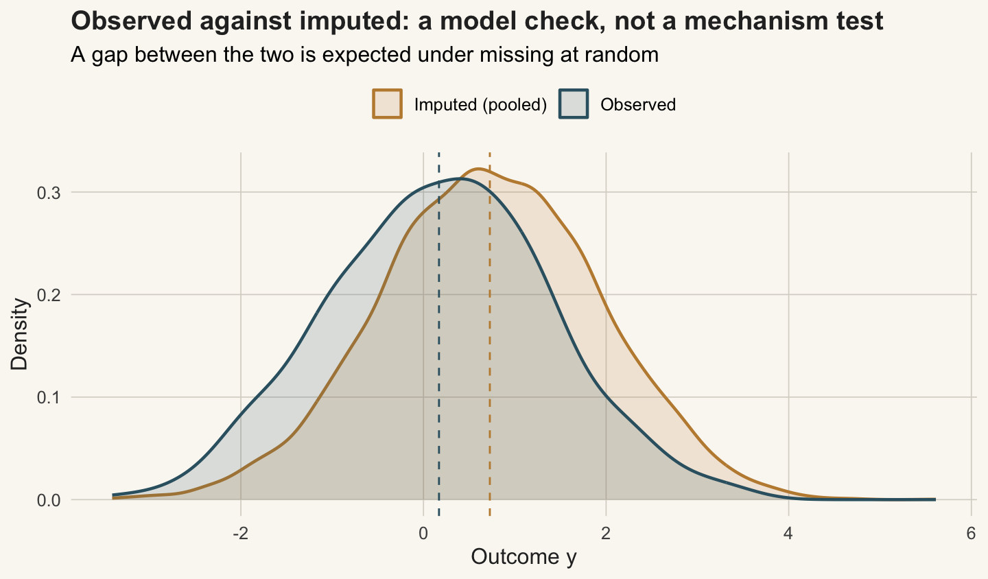
The next instinct is to compare the values the imputation invents against the values that were seen, and worry if they differ. Figure 1 shows that comparison.
```{r}
#| label: fig-obs-imp
#| fig-cap: "The distribution of observed outcomes against the pooled distribution of imputed outcomes. The imputed values sit higher because the missing rows have higher x; under missing at random that shift is expected, and its presence is not evidence against the imputation."
#| fig-alt: "Two overlaid densities of the outcome. The imputed distribution sits to the right of the observed distribution, with their means marked by dashed lines a short distance apart."
#| fig-width: 7.5
#| fig-height: 4.4
obs_y <- y[!my]; imp_y <- unlist(lapply(imps, function(v) v[my]))
df1 <- rbind(data.frame(y = obs_y, src = "Observed"),
             data.frame(y = imp_y, src = "Imputed (pooled)"))
mu1 <- df1 |> group_by(src) |> summarise(m = mean(y), .groups = "drop")
ggplot(df1, aes(y, colour = src, fill = src)) +
  geom_density(alpha = 0.16, linewidth = 0.8) +
  geom_vline(data = mu1, aes(xintercept = m, colour = src),
             linetype = "dashed", linewidth = 0.5, show.legend = FALSE) +
  scale_colour_manual(values = c("Observed" = "#356170", "Imputed (pooled)" = "#c08a3e")) +
  scale_fill_manual(values = c("Observed" = "#356170", "Imputed (pooled)" = "#c08a3e")) +
  labs(title = "Observed against imputed: a model check, not a mechanism test",
       subtitle = "A gap between the two is expected under missing at random",
       x = "Outcome y", y = "Density", colour = NULL, fill = NULL) + theme_te()
```
The imputed outcomes sit a little above the observed ones. It is tempting to read that as a problem, but it is not: the missing rows are the high-`x` rows, and higher `x` means a higher `y`, so an imputation that is working *should* place them higher. A diagnostic like this earns its keep by catching imputations that are plainly wrong, values outside the possible range, a bimodal shape where the data are unimodal, impossible negative counts. It confirms the imputation model is behaving. It says nothing about whether the mechanism is missing at random, because both mechanisms are consistent with this picture.
## Probing the mechanism with a delta shift
If the assumption cannot be tested, the remaining move is to break it deliberately and watch. Suppose the outcomes are missing not at random in the worst plausible way: the units in the treatment group whose outcome went missing did so *because* they were doing badly, so their true outcomes are lower than a missing-at-random imputation assumes, by some amount delta. Shift every imputed treatment-group outcome down by delta, re-pool, and sweep delta across a range. This is a pattern-mixture, or delta-adjustment, sensitivity analysis.
```{r}
#| label: delta-sweep
deltas <- seq(0, 1.5, 0.025)
trtmiss <- my & (g == 1)
sweep <- t(sapply(deltas, function(dl) {
  ests <- ses <- numeric(m)
  for (k in 1:m) { yc <- imps[[k]]; yc[trtmiss] <- yc[trtmiss] - dl
    e <- eff(yc); ests[k] <- e[1]; ses[k] <- e[2] }
  p <- pool(ests, ses, m, nu_com); tc <- qt(0.975, p["df"])
  c(delta = dl, est = p["Q"], lo = p["Q"] - tc * p["se"], hi = p["Q"] + tc * p["se"])
}))
sweep <- as.data.frame(sweep); colnames(sweep) <- c("delta", "est", "lo", "hi")
tip <- sweep$delta[which(sweep$lo <= 0)[1]]
c(mar_effect = round(sweep$est[1], 3), tipping_delta = round(tip, 3),
  outcome_sd = round(sd(y_true), 3), tipping_in_outcome_sd = round(tip / sd(y_true), 3))
```
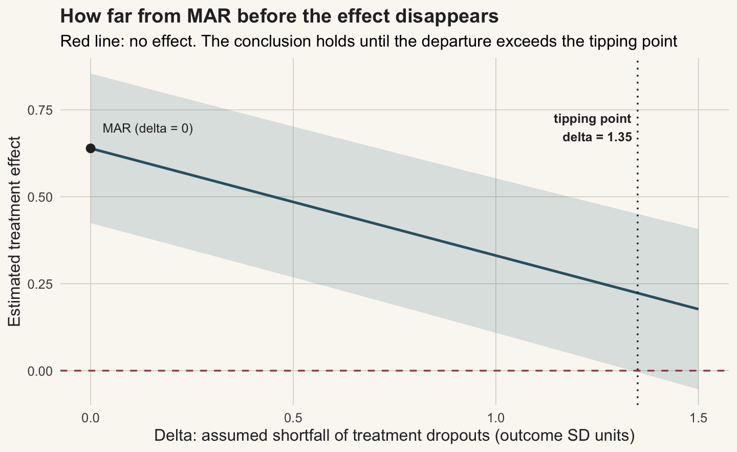
At delta zero (missing at random) the effect is `r round(sweep$est[1], 3)`. As the assumed shortfall grows, the effect shrinks steadily: `r round(sweep$est[which.min(abs(sweep$delta-0.5))],3)` at a shift of half an outcome unit, `r round(sweep$est[which.min(abs(sweep$delta-1.0))],3)` at a full one. The interval first touches zero at a delta of `r round(tip, 2)`. Figure 2 traces the whole path.
```{r}
#| label: fig-sensitivity
#| fig-cap: "The estimated treatment effect and its 95% interval as the assumed departure from missing at random grows. The effect stays clear of zero until the treatment dropouts are assumed to fall short by more than the tipping-point delta."
#| fig-alt: "A downward sloping line with a shaded interval, starting near 0.64 at delta zero and falling steadily without reaching zero, while the lower edge of its shaded interval first touches the zero line at a delta of about 1.35, marked with a dotted vertical line."
#| fig-width: 7.5
#| fig-height: 4.6
p_sens <- ggplot(sweep, aes(delta, est)) +
  geom_ribbon(aes(ymin = lo, ymax = hi), fill = "#4a7a8c", alpha = 0.18) +
  geom_line(colour = "#356170", linewidth = 0.9) +
  geom_hline(yintercept = 0, colour = "#a24b4b", linetype = "dashed", linewidth = 0.6) +
  geom_vline(xintercept = tip, colour = ink, linetype = "dotted", linewidth = 0.6) +
  annotate("point", x = 0, y = sweep$est[1], colour = ink, size = 2.6) +
  annotate("text", x = 0.03, y = sweep$est[1] + 0.06, label = "MAR (delta = 0)",
           hjust = 0, size = 3.3, colour = ink) +
  annotate("text", x = tip, y = 0.7, label = sprintf("tipping point\ndelta = %.2f", tip),
           hjust = 1.08, size = 3.3, colour = ink, fontface = "bold") +
  labs(title = "How far from MAR before the effect disappears",
       subtitle = "Red line: no effect. The conclusion holds until the departure exceeds the tipping point",
       x = "Delta: assumed shortfall of treatment dropouts (outcome units)",
       y = "Estimated treatment effect") + theme_te()
p_sens
```
```{r}
#| label: thumb
#| include: false
ggsave("thumbnail.png",
p_sens + labs(title = NULL, subtitle = NULL) +
theme(plot.margin = margin(8, 14, 8, 8)),
width = 7.5, height = 5.4, dpi = 100, bg = paper)
```
## The honest limit
The tipping point is the whole point. The data cannot tell you the true delta, so a sensitivity analysis does not resolve the question; it relocates it. Instead of an untestable yes-or-no about missing at random, you are left with a quantity you can reason about: the treatment effect survives unless the dropouts in the treatment arm were doing worse than a missing-at-random imputation assumes by more than `r round(tip, 2)` units of the outcome, which is `r round(tip / sd(y_true), 2)` standard deviations of it. That is a large and specific departure, and whether it is plausible is a question for what is known about the study and its dropouts, not for the dataset. A small tipping point would be a warning that the conclusion rests on the assumption; a large one, as here, is reassurance that it does not rest on it much.
This is the same move that closes the measurement-error and causal-inference threads on this blog. None of them makes an untestable assumption testable. What they do is convert it into a magnitude, quantify how large a violation the conclusion could absorb, and hand that number back to the reader to judge. For missing data specifically: check the model with diagnostics, reject complete randomness where you can, and then report the tipping point rather than a bare interval that hides the assumption it depends on. If a real decision turns on the result, the delta you are willing to defend is part of the analysis, not an afterthought.
## References
Rubin DB 1976. Biometrika 63(3):581-592 (10.1093/biomet/63.3.581).
Little RJA 1988. Journal of the American Statistical Association 83(404):1198-1202 (10.1080/01621459.1988.10478722).
Little RJA 1993. Journal of the American Statistical Association 88(421):125-134 (10.1080/01621459.1993.10594302).
van Buuren S 2018. Flexible Imputation of Missing Data, 2nd edn. Chapman and Hall/CRC (10.1201/9780429492259).
Carpenter JR, Kenward MG 2013. Multiple Imputation and its Application. Wiley. ISBN 978-0-470-74052-1.
Molenberghs G, Kenward MG 2007. Missing Data in Clinical Studies. Wiley. ISBN 978-0-470-84981-1.
National Research Council 2010. The Prevention and Treatment of Missing Data in Clinical Trials. National Academies Press. ISBN 978-0-309-15814-5.
Johnson TF, Isaac NJB, Paviolo A, Gonzalez-Suarez M 2021. Global Ecology and Biogeography 30(1):51-62 (10.1111/geb.13185).
## Related tutorials
- [Missing data: MCAR, MAR and MNAR](../missing-data-mechanisms-mcar-mar-mnar/)
- [Single imputation: bias and variance](../single-imputation-bias-variance/)
- [Multiple imputation by chained equations](../multiple-imputation-chained-equations/)
- [Missing values in a predictor: why, not how many](../missing-values-in-a-predictor/)