---
title: "Multiple imputation by chained equations"
description: "Multiple imputation coded by hand in R, with chained equations and Rubin's rules: an unbiased slope and an honest standard error where single imputation fails."
date: "2026-05-28 12:00"
categories: [R, missing data, simulation, ggplot2, ecology tutorial]
image: thumbnail.png
image-alt: "A caterpillar plot of fifty imputation slope estimates in blue with a wider red pooled interval below them, marked against the true value."
---
The previous post ended on a wall: even a well-built single imputation reports too little uncertainty, because one completed dataset treats the filled values as if they were real. Multiple imputation walks around the wall instead of over it. Rather than commit to one set of guesses, it draws several completed datasets, analyses each, and then lets the disagreement between them widen the standard error. This post builds the method by hand, chained equations for the imputation and Rubin's rules for the pooling, and checks that it delivers what single imputation could not.
The example has two variables with gaps, `x` and `y`, and a fully observed auxiliary `z` that helps predict them. The target is the slope of `y` on `x`, whose true value is 0.8.
```{r}
#| label: setup
#| message: false
#| warning: false
#| code-fold: true
#| code-summary: "Setup: packages, colours and plot theme"
library(ggplot2); library(dplyr); library(tidyr); library(MASS)
ink <- "#2b2b2b"; grid_col <- "#d9d5cc"; paper <- "#f5f4ee"
theme_te <- function(base = 12) {
  theme_minimal(base_size = base) +
    theme(panel.grid.minor = element_blank(),
          panel.grid.major = element_line(colour = grid_col, linewidth = 0.3),
          plot.background = element_rect(fill = paper, colour = NA),
          panel.background = element_rect(fill = paper, colour = NA),
          strip.text = element_text(face = "bold", colour = ink),
          plot.title = element_text(face = "bold", colour = ink),
          axis.title = element_text(colour = ink),
          legend.position = "top")
}
```
## One proper imputation step
Chained equations fill one variable at a time. To impute a variable from a set of predictors, fit a linear model on the rows where it is observed, then draw fresh values for the gaps from the model's predictive distribution. The word *proper* matters: a single stochastic imputation used the point estimates of the regression coefficients and the residual scale, which understates uncertainty. Here we draw the residual variance and the coefficients from their posterior first, so that each imputation reflects the fact that the imputation model is itself estimated.
```{r}
#| label: step-fn
## draw sigma^2 from its scaled inverse chi-square posterior, then beta given sigma^2,
## then fill the gaps with the predicted mean plus a residual draw
step <- function(target, mask, preds) {
  obs <- !mask
  Xo <- cbind(1, preds[obs, , drop = FALSE]); Vo <- target[obs]
  XtXinv <- chol2inv(chol(crossprod(Xo)))
  bhat <- XtXinv %*% crossprod(Xo, Vo)
  dfree <- sum(obs) - ncol(Xo)
  s2 <- sum((Vo - Xo %*% bhat)^2) / dfree
  s2star <- s2 * dfree / rchisq(1, dfree)                    # posterior draw of variance
  bstar <- bhat + t(chol(s2star * XtXinv)) %*% rnorm(ncol(Xo))  # posterior draw of coefficients
  out <- target
  Xm <- cbind(1, preds[mask, , drop = FALSE])
  out[mask] <- as.numeric(Xm %*% bstar) + rnorm(sum(mask), 0, sqrt(s2star))
  out
}
```
## Chaining the variables
With more than one incomplete variable, no single regression has all its predictors observed, so the method cycles. Start by filling every gap with a random observed value, then repeatedly re-impute each variable using the current version of the others. A handful of cycles is enough for the fills to settle.
```{r}
#| label: chain-fn
one_impute <- function(x, y, z, mx, my, cycles = 5) {
  xc <- x; xc[mx] <- sample(x[!mx], sum(mx), TRUE)   # random start
  yc <- y; yc[my] <- sample(y[!my], sum(my), TRUE)
  for (c in seq_len(cycles)) {
    xc <- step(x, mx, cbind(yc, z))                  # x given current y and z
    yc <- step(y, my, cbind(xc, z))                  # y given current x and z
  }
  data.frame(x = xc, y = yc)
}
```
## The data
```{r}
#| label: dgp
set.seed(5108)
n <- 400
z <- rnorm(n)
x_true <- 0.7 * z + rnorm(n, 0, sqrt(1 - 0.49))         # x correlated with z
y_true <- 1 + 0.8 * x_true + rnorm(n, 0, 1.2)           # slope of interest is 0.8
## missing at random: high z makes both x and y more likely to be missing (about 30% each)
ax <- uniroot(function(a) mean(plogis(a + z)) - 0.30, c(-6, 6))$root
mx <- runif(n) < plogis(ax + z)
my <- runif(n) < plogis(ax + z)
x <- x_true; x[mx] <- NA
y <- y_true; y[my] <- NA

full <- lm(y_true ~ x_true)
full_b <- unname(coef(full)[2]); full_se <- summary(full)$coef[2, 2]
cc <- !mx & !my
ccf <- lm(y[cc] ~ x[cc])
cc_b <- unname(coef(ccf)[2]); cc_se <- summary(ccf)$coef[2, 2]
```
About `r round(100 * mean(mx))`% of `x` and `r round(100 * mean(my))`% of `y` are missing, and only `r sum(cc)` of the `r n` rows have both. The full data (which we only have here because it is a simulation) give a slope of `r round(full_b, 3)` with a standard error of `r round(full_se, 3)`. Complete-case analysis, on those `r sum(cc)` rows, gives `r round(cc_b, 3)` with a standard error of `r round(cc_se, 3)`: unbiased by design here, but wide, because it throws away every partially observed row.
## Many imputations, then Rubin's rules
Run the chained imputation `r 50` times to build 50 completed datasets, fit the slope on each, and collect the estimates and their standard errors.
```{r}
#| label: many
m <- 50
ests <- ses <- numeric(m)
for (k in 1:m) {
  d <- one_impute(x, y, z, mx, my, cycles = 5)
  f <- lm(y ~ x, data = d)
  ests[k] <- coef(f)[2]; ses[k] <- summary(f)$coef[2, 2]
}
```
Rubin's rules combine the `m` results. The pooled estimate is the average of the per-imputation estimates. The total variance has two parts: the average within-imputation variance (the ordinary uncertainty had the data been complete), plus the between-imputation variance (the extra uncertainty from not knowing the missing values), inflated by a factor `1 + 1/m`.
```{r}
#| label: rubin
pool <- function(ests, ses, m, nu_com) {
  Qbar <- mean(ests)                       # pooled estimate
  Ubar <- mean(ses^2)                      # within-imputation variance
  B <- var(ests)                           # between-imputation variance
  Tt <- Ubar + (1 + 1 / m) * B             # total variance
  lambda <- (1 + 1 / m) * B / Tt           # fraction of missing information
  nu_old <- (m - 1) / lambda^2
  nu_obs <- (nu_com + 1) / (nu_com + 3) * nu_com * (1 - lambda)
  df <- nu_old * nu_obs / (nu_old + nu_obs) # Barnard-Rubin degrees of freedom
  c(Q = Qbar, se = sqrt(Tt), B = B, Ubar = Ubar, lambda = lambda, df = df)
}
pl <- pool(ests, ses, m, nu_com = n - 2)
round(pl, 4)
```
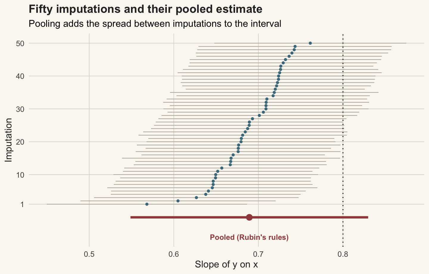
The pooled slope is `r round(pl["Q"], 3)`, with a standard error of `r round(pl["se"], 3)` on `r round(pl["df"], 1)` degrees of freedom. In this particular sample the complete cases already sit low, near `r round(cc_b, 2)`, so multiple imputation stays close to that rather than inventing a stronger relationship; the simulation below confirms all three estimators are unbiased on average. The between-imputation variance is `r round(pl["B"], 4)`, small next to the within-imputation `r round(pl["Ubar"], 4)`, and the fraction of missing information is `r round(pl["lambda"], 3)`: roughly a third of the information about this slope is lost to the gaps. Figure 1 lays out the 50 imputations and their pooled summary.
```{r}
#| label: fig-caterpillar
#| fig-cap: "The fifty per-imputation slope estimates and their 95% intervals, with the Rubin-pooled estimate below. The pooled interval is wider than any single one, because it adds the between-imputation variance. The dotted line is the true slope."
#| fig-alt: "A caterpillar plot: fifty blue points with horizontal intervals scattered around 0.7, and a single red pooled point below them with a wider interval, against a dotted line at 0.8."
#| fig-width: 7.5
#| fig-height: 4.8
ord <- order(ests)
cap <- data.frame(idx = 1:m, est = ests[ord], lo = ests[ord] - 1.96 * ses[ord],
                  hi = ests[ord] + 1.96 * ses[ord])
tcrit <- qt(0.975, pl["df"])
lo_p <- pl["Q"] - tcrit * pl["se"]; hi_p <- pl["Q"] + tcrit * pl["se"]
ggplot(cap, aes(y = idx)) +
  geom_segment(aes(x = lo, xend = hi, yend = idx), colour = "#b9b4a8", linewidth = 0.4) +
  geom_point(aes(x = est), colour = "#4a7a8c", size = 1.1) +
  geom_vline(xintercept = 0.8, colour = ink, linetype = "dotted", linewidth = 0.6) +
  annotate("segment", x = lo_p, xend = hi_p, y = -3, yend = -3, colour = "#a24b4b", linewidth = 1.4) +
  annotate("point", x = pl["Q"], y = -3, colour = "#a24b4b", size = 3.2) +
  annotate("text", x = pl["Q"], y = -9, label = "Pooled (Rubin's rules)",
           colour = "#a24b4b", size = 3.3, fontface = "bold") +
  scale_y_continuous(breaks = c(1, 10, 20, 30, 40, 50)) +
  labs(title = "Fifty imputations and their pooled estimate",
       subtitle = "Pooling adds the spread between imputations to the interval",
       x = "Slope of y on x", y = "Imputation") + theme_te()
```
## Does it cover?
The single dataset is suggestive, not proof. Repeat the whole pipeline over many datasets and compare three estimators: complete-case, a single stochastic imputation, and pooled multiple imputation. Record whether each 95% interval covers the truth and how wide it is.
```{r}
#| label: monte-carlo
reps <- 400; mM <- 20; b1 <- 0.8
res <- matrix(NA, reps, 7,
  dimnames = list(NULL, c("cc_b", "cc_cov", "cc_w", "si_cov", "si_w", "mi_cov", "mi_w")))
si_b <- mi_b <- numeric(reps)
set.seed(909)
for (r in 1:reps) {
  zz <- rnorm(n); xt <- 0.7 * zz + rnorm(n, 0, sqrt(1 - 0.49))
  yt <- 1 + 0.8 * xt + rnorm(n, 0, 1.2)
  a <- uniroot(function(a) mean(plogis(a + zz)) - 0.30, c(-6, 6))$root
  mxx <- runif(n) < plogis(a + zz); myy <- runif(n) < plogis(a + zz)
  xx <- xt; xx[mxx] <- NA; yy <- yt; yy[myy] <- NA
  cr <- !mxx & !myy; cf <- lm(yy[cr] ~ xx[cr]); cb <- coef(cf)[2]; cs <- summary(cf)$coef[2, 2]
  res[r, "cc_b"] <- cb; res[r, "cc_w"] <- 2 * 1.96 * cs
  res[r, "cc_cov"] <- (cb - 1.96 * cs <= b1) & (b1 <= cb + 1.96 * cs)
  es <- ss <- numeric(mM)
  for (k in 1:mM) { d <- one_impute(xx, yy, zz, mxx, myy, cycles = 4)
    f <- lm(y ~ x, data = d); es[k] <- coef(f)[2]; ss[k] <- summary(f)$coef[2, 2] }
  si_b[r] <- es[1]
  res[r, "si_cov"] <- (es[1] - 1.96 * ss[1] <= b1) & (b1 <= es[1] + 1.96 * ss[1])
  res[r, "si_w"] <- 2 * 1.96 * ss[1]
  p <- pool(es, ss, mM, n - 2); tc <- qt(0.975, p["df"])
  mi_b[r] <- p["Q"]
  res[r, "mi_cov"] <- (p["Q"] - tc * p["se"] <= b1) & (b1 <= p["Q"] + tc * p["se"])
  res[r, "mi_w"] <- 2 * tc * p["se"]
}
tab <- data.frame(
  method = c("Complete-case", "Single imputation", "Multiple imputation"),
  bias = c(mean(res[, "cc_b"]) - b1, mean(si_b) - b1, mean(mi_b) - b1),
  coverage = c(mean(res[, "cc_cov"]), mean(res[, "si_cov"]), mean(res[, "mi_cov"])),
  width = c(mean(res[, "cc_w"]), mean(res[, "si_w"]), mean(res[, "mi_w"])))
round(tab[, -1], 3)
```
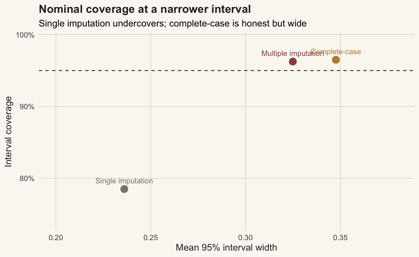
All three are unbiased, each within `r sprintf("%.3f", max(abs(c(mean(res[,"cc_b"]),mean(si_b),mean(mi_b))-b1)))` of the true 0.8. The difference is in the intervals. Complete-case covers at `r round(100*mean(res[,"cc_cov"]))`%, honestly, but its mean width is `r round(mean(res[,"cc_w"]),3)`. Single imputation covers at only `r round(100*mean(res[,"si_cov"]))`%, the undercoverage carried over from the last post. Multiple imputation covers at `r round(100*mean(res[,"mi_cov"]))`% with a mean width of `r round(mean(res[,"mi_w"]),3)`, narrower than complete-case because it uses the partially observed rows through the auxiliary `z`. Figure 2 places the three on the same axes.
```{r}
#| label: fig-coverage
#| fig-cap: "Interval coverage against mean interval width for the three estimators. The dashed line is the 95% target. Multiple imputation reaches it at a narrower width than complete-case, while single imputation falls short."
#| fig-alt: "A scatter of coverage against interval width. Multiple imputation sits near 95% at a narrow width, complete-case near 95% but wider, and single imputation well below 95%."
#| fig-width: 7.5
#| fig-height: 4.6
sm <- data.frame(method = factor(c("Complete-case", "Single imputation", "Multiple imputation"),
                                 levels = c("Complete-case", "Single imputation", "Multiple imputation")),
                 coverage = c(mean(res[, "cc_cov"]), mean(res[, "si_cov"]), mean(res[, "mi_cov"])),
                 width = c(mean(res[, "cc_w"]), mean(res[, "si_w"]), mean(res[, "mi_w"])))
ggplot(sm, aes(width, coverage, colour = method)) +
  geom_hline(yintercept = 0.95, colour = ink, linetype = "dashed", linewidth = 0.5) +
  geom_point(size = 4) +
  geom_text(aes(label = method), size = 3.4, show.legend = FALSE,
            hjust = ifelse(sm$method == "Multiple imputation", 1.08, 0.5),
            vjust = ifelse(sm$method == "Multiple imputation", 0.5, -1.1)) +
  scale_colour_manual(values = c("Complete-case" = "#c08a3e",
                                 "Single imputation" = "#8a8578",
                                 "Multiple imputation" = "#a24b4b"), guide = "none") +
  scale_y_continuous(labels = function(v) paste0(round(100 * v), "%")) +
  coord_cartesian(xlim = c(0.2, 0.38), ylim = c(0.74, 0.99)) +
  labs(title = "Nominal coverage at a narrower interval",
       subtitle = "Single imputation undercovers; complete-case is honest but wide",
       x = "Mean 95% interval width", y = "Interval coverage") + theme_te()
```
## The honest limit
Multiple imputation is not magic, and it is worth being clear about what carries it. The between-imputation variance is an honest accounting of one specific uncertainty: not knowing the missing values, *given* that the imputation model is right and the data are missing at random. It does nothing about the mechanism. If the gaps are missing not at random, every imputation is drawn from the wrong distribution and the pooled interval is confidently wrong, just as complete-case would be. It also assumes the imputation model and the analysis model tell a consistent story; when they do not, the pooled variance can be too small or too large (Meng 1994). Raising the number of imputations shrinks the Monte Carlo noise in the pooling, but it cannot fix a wrong model or a wrong mechanism, only sharpen the answer to the question actually posed. The working assumption throughout has been missing at random. The final post asks how to probe it, and what to do when it is indefensible.
## References
Rubin DB 1987. Multiple Imputation for Nonresponse in Surveys. Wiley. ISBN 978-0-471-08705-2.
Rubin DB 1996. Journal of the American Statistical Association 91(434):473-489 (10.1080/01621459.1996.10476908).
van Buuren S, Groothuis-Oudshoorn K 2011. Journal of Statistical Software 45(3):1-67 (10.18637/jss.v045.i03).
White IR, Royston P, Wood AM 2011. Statistics in Medicine 30(4):377-399 (10.1002/sim.4067).
Barnard J, Rubin DB 1999. Biometrika 86(4):948-955 (10.1093/biomet/86.4.948).
Meng XL 1994. Statistical Science 9(4):538-558 (10.1214/ss/1177010269).
Penone C, Davidson AD, Shoemaker KT, Di Marco M, Rondinini C, Brooks TM, Young BE, Graham CH, Costa GC 2014. Methods in Ecology and Evolution 5(9):961-970 (10.1111/2041-210X.12232).
van Buuren S 2018. Flexible Imputation of Missing Data, 2nd edn. Chapman and Hall/CRC (10.1201/9780429492259).
## Related tutorials
- [Missing data: MCAR, MAR and MNAR](../missing-data-mechanisms-mcar-mar-mnar/)
- [Single imputation: bias and variance](../single-imputation-bias-variance/)
- [Checking missing-data assumptions](../checking-missing-data-assumptions/)
- [Missing values in a predictor: why, not how many](../missing-values-in-a-predictor/)