Checking a measurement-error correction

The measurement-error toolkit assumes you know the error size. Here: estimating reliability from replicates, checking whether to correct, and sensitivity analysis.

Every correction in this cluster took one number as given. The moment correction divided by the reliability. Deming regression asked for the ratio of the two error variances. SIMEX calibrated its whole simulation in multiples of the measurement-error variance. None of them can start without a number describing how large the error is, and none of them can recover that number from the error-prone data alone. This closing post is about where the number comes from, whether the correction is worth making once you have it, and what to do when you cannot get it at all.

Estimating reliability from repeated measurements

The clean way to learn the size of measurement error is to measure the same units more than once. If you weigh each animal three times, or send each soil sample to the lab in triplicate, the spread within a unit is measurement error and the spread between units is real variation. A one-way analysis of variance separates the two.

set.seed(7314)
m   <- 80                         # units measured repeatedly
r   <- 3                          # measurements per unit
sdx <- 3; sdu <- 2                # true between-unit sd 3, error sd 2

xt  <- rnorm(m, 10, sdx)          # latent true value of each unit
dat <- data.frame(
  unit = factor(rep(1:m, each = r)),
  w    = rep(xt, each = r) + rnorm(m * r, 0, sdu)
)

fit  <- aov(w ~ unit, data = dat)
ms   <- summary(fit)[[1]][, "Mean Sq"]
ms_b <- ms[1]; ms_w <- ms[2]

var_u_hat <- ms_w                 # within-unit mean square estimates error variance
var_x_hat <- (ms_b - ms_w) / r    # between minus within, scaled, estimates true variance
icc       <- var_x_hat / (var_x_hat + var_u_hat)

The within-unit mean square estimates the measurement-error variance directly, at 4.3 against a true value of 4. The between-unit component recovers 11.08 for a true 9. Their ratio is the reliability, here 0.72 against a true 0.692. This quantity is the intraclass correlation coefficient, and it is exactly the reliability the first post divided by. The estimate carries its own sampling error, wider for the between-unit part because it rests on only 80 unit means, which is itself worth remembering: the reliability you plug into a correction is a guess with a confidence interval, not a constant.

Replicates buy a second thing. Averaging the 3 measurements per unit gives a predictor whose error variance is smaller by a factor of 3, lifting its reliability from about 0.72 for a single reading to 0.885 for the mean. Measuring twice and averaging is often a cheaper route to a usable predictor than any correction applied afterwards.

Is the correction worth making?

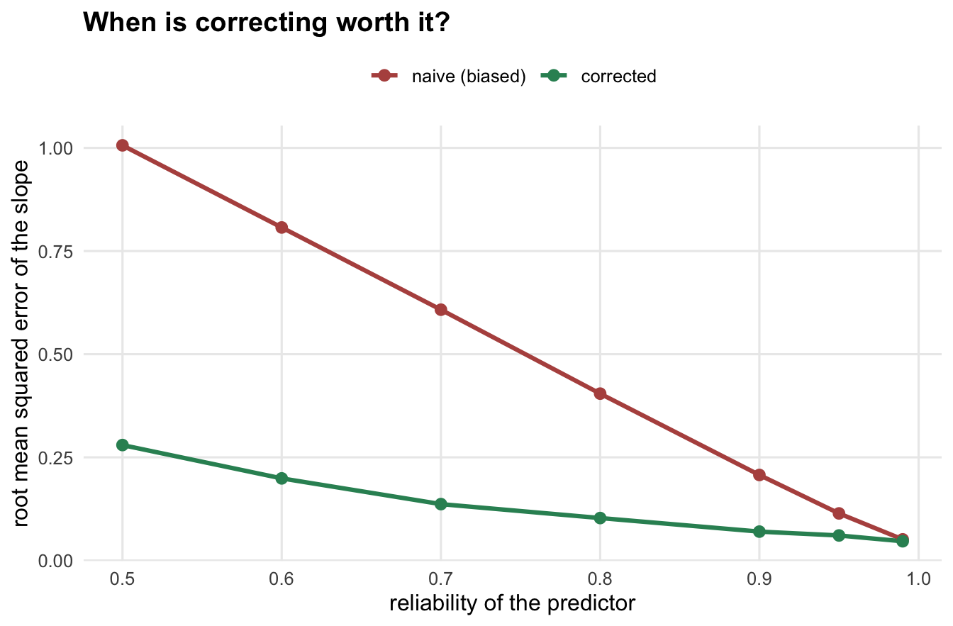
A correction is not free. It removes bias, but it inflates the variance of the estimate, because it divides by a reliability that is itself estimated and less than one. When the error is small the bias it removes is tiny, and the variance it adds can leave you worse off than doing nothing. The way to see the trade is to compare the naive and corrected slopes by root mean squared error, which folds bias and variance into one number, across a range of reliabilities.

b1 <- 2; b0 <- 1; n <- 200; sde <- 2; sdx2 <- 3; varx <- sdx2^2
rel_levels <- c(0.5, 0.6, 0.7, 0.8, 0.9, 0.95, 0.99)
reps <- 600

res <- data.frame()
set.seed(202)
for (rel in rel_levels) {
  varu <- varx * (1 - rel) / rel
  bn <- numeric(reps); bc <- numeric(reps)
  for (k in seq_len(reps)) {
    x <- rnorm(n, 10, sdx2)
    y <- b0 + b1 * x + rnorm(n, 0, sde)
    w <- x + rnorm(n, 0, sqrt(varu))
    bn[k] <- coef(lm(y ~ w))[2]
    lam   <- (var(w) - varu) / var(w)
    bc[k] <- bn[k] / lam
  }
  res <- rbind(res, data.frame(rel,
    rmse_naive = sqrt(mean((bn - b1)^2)),
    rmse_corr  = sqrt(mean((bc - b1)^2))))
}

At a reliability of 0.5 the naive slope is badly biased and its error is 1.006, while the corrected slope cuts that to 0.28: correcting is clearly worth it. At a reliability of 0.99 the picture reverses in spirit. The naive error is already down to 0.051, and the corrected version, at 0.047, is no better, because there was almost no bias to remove and the correction only added noise. The variance cost is always present; it is worth paying only when it buys a real reduction in bias.

d1 <- pivot_longer(res, c(rmse_naive, rmse_corr),
                   names_to = "estimator", values_to = "rmse")
d1$estimator <- factor(d1$estimator, levels = c("rmse_naive", "rmse_corr"),
                       labels = c("naive (biased)", "corrected"))
ggplot(d1, aes(rel, rmse, colour = estimator)) +
  geom_line(linewidth = 1.1) + geom_point(size = 2.4) +
  scale_colour_manual(values = c("naive (biased)" = col_naive, "corrected" = col_corr),
                      name = NULL) +
  labs(title = "When is correcting worth it?",
       x = "reliability of the predictor",
       y = "root mean squared error of the slope") +
  theme_te

Figure 1: Root mean squared error of the slope against the reliability of the predictor, for the naive estimate (red) and the moment-corrected estimate (green). Correction wins decisively when reliability is low, but the two converge as reliability approaches one, where the correction adds variance without removing meaningful bias.

When you cannot measure the error

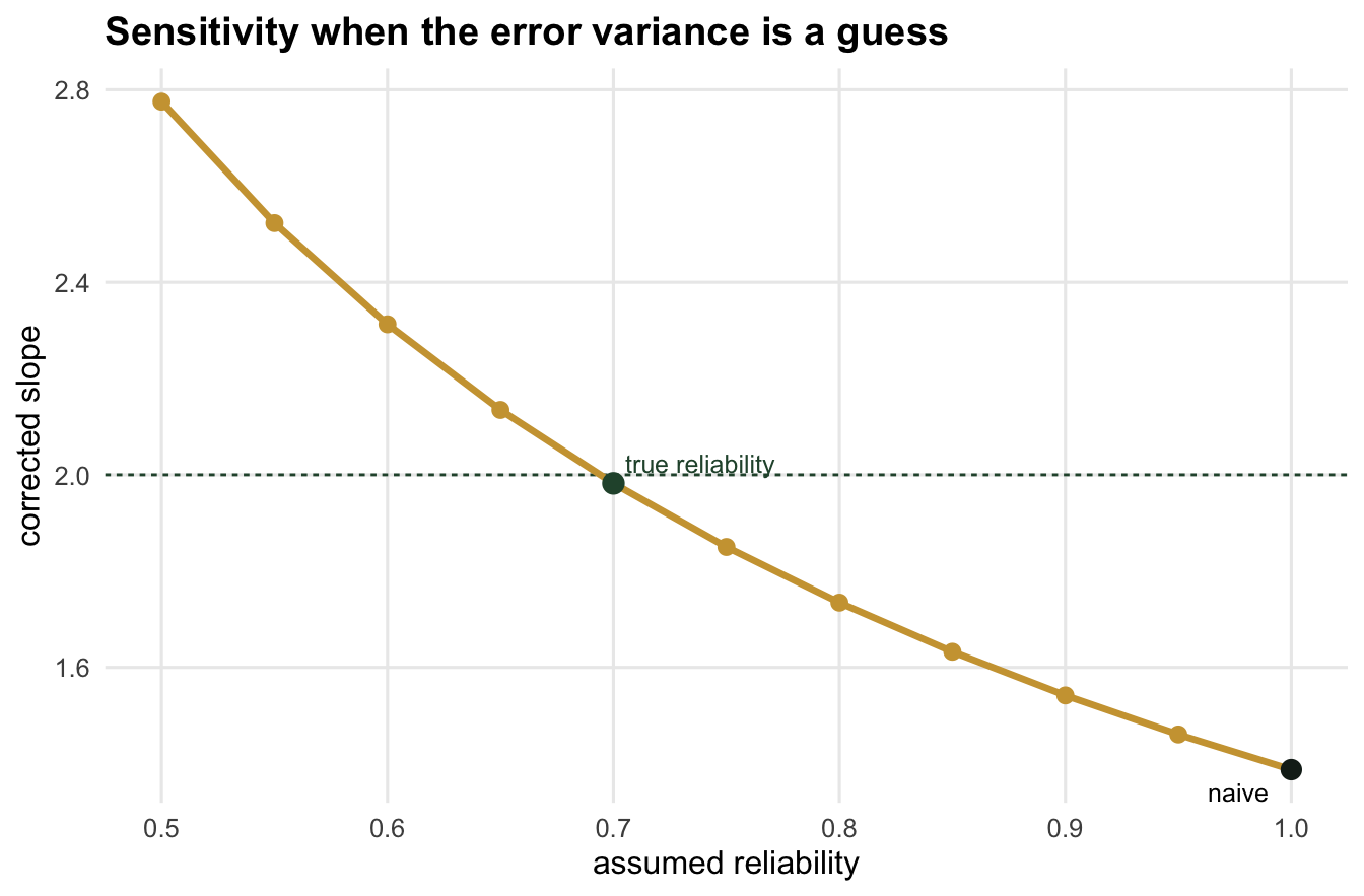
Sometimes there are no replicates and no validation sample, and the error variance is genuinely unknown. You are not stuck, but you cannot produce a single corrected number and call it the answer. What you can do is show how the corrected estimate moves as the assumed reliability moves, and let the reader see the dependence rather than hiding it.

set.seed(551)
rel_true  <- 0.7
varu_true <- varx * (1 - rel_true) / rel_true
x <- rnorm(n, 10, sdx2)
y <- b0 + b1 * x + rnorm(n, 0, sde)
w <- x + rnorm(n, 0, sqrt(varu_true))

b_naive <- coef(lm(y ~ w))[2]
assumed_rel <- seq(0.5, 1.0, by = 0.05)
corrected   <- b_naive / assumed_rel        # correction under each assumed reliability

The naive slope is 1.388. Sweeping the assumed reliability from 0.5 to 1.0 sends the corrected slope from 2.775 down to 1.388, the latter being just the naive value when you assume no error at all. Only at the true reliability of 0.7 does the correction land near the real slope, at 1.982. The band is wide, and that width is the honest result: with an unknown error variance the data are consistent with a broad range of slopes, and the right output is that range together with a statement of what reliability each end assumes.

sens <- data.frame(assumed_rel, corrected)
ggplot(sens, aes(assumed_rel, corrected)) +
  geom_hline(yintercept = b1, colour = col_true, linewidth = 0.5, linetype = "22") +
  geom_line(colour = col_acc, linewidth = 1.2) +
  geom_point(colour = col_acc, size = 2.4) +
  annotate("point", x = 1.0, y = b_naive, colour = "#16241d", size = 3) +
  annotate("point", x = rel_true, y = b_naive / rel_true, colour = col_true, size = 3.2) +
  annotate("text", x = 0.99, y = b_naive, label = "naive\n(assume no error)",
           hjust = 1, vjust = 1.3, size = 3.3, lineheight = 0.9) +
  annotate("text", x = rel_true, y = b_naive / rel_true, label = "true reliability",
           hjust = -0.08, vjust = -0.6, size = 3.3, colour = col_true) +
  labs(title = "Sensitivity when the error variance is a guess",
       x = "assumed reliability", y = "corrected slope") +
  theme_te

Figure 2: The corrected slope as a function of the reliability you assume, for a single dataset. The dashed line is the true slope; the dark point on the right is the naive estimate, which assumes no error; the green point marks the true reliability. Without external information to fix the reliability, the whole curve is admissible.

What to take away

Measurement-error correction is only as trustworthy as the error information behind it. If you can measure the same units more than once, one-way analysis of variance turns the replicates into a reliability estimate and, by averaging, into a better predictor at the same time. Before reaching for any correction, ask whether it is worth it: at high reliability the bias is small and the correction mostly adds variance, so the honest move is to leave the estimate alone. And when the error variance cannot be pinned down, do not manufacture a single corrected figure. Report the corrected estimate across a plausible range of reliabilities and state the assumption at each end, so the reader can judge how much the conclusion leans on a number you had to guess.

That is the thread running through the whole cluster. Regression dilution, errors-in-variables, and SIMEX are different machines for the same task, and each needs to be told how large the error is. The measurement of the measurement error is not a preliminary to the analysis; it is the part that makes the analysis possible.

References

• Fuller 1987 Measurement Error Models, ISBN 978-0-471-86187-4
• Carroll, Ruppert, Stefanski, Crainiceanu 2006 Measurement Error in Nonlinear Models, 2nd ed, ISBN 978-1-58488-633-4
• Nakagawa, Schielzeth 2010 Biological Reviews 85(4):935-956 (10.1111/j.1469-185X.2010.00141.x)
• Bartlett, Keogh 2018 Statistical Methods in Medical Research 27(6):1695-1708 (10.1177/0962280216667764)

Related tutorials

• Measurement error and regression dilution
• Errors-in-variables and Deming regression
• Correcting measurement error with SIMEX
• Standard errors and confidence intervals