Errors-in-variables and Deming regression

When both variables carry error, ordinary regression is biased either way. Deming regression uses the error-variance ratio to recover the true slope in R.

Updated 27 September 2026: a new section, Two methods on one scale, measures how often a Bland-Altman plot reports proportional bias between two unbiased methods of unequal precision, and what a Deming check needs from repeat measurements to avoid the same mistake.

The previous post put measurement error on one variable and watched the slope shrink. Field data rarely obliges by keeping one axis clean. Compare two field methods for canopy cover and both are noisy. Calibrate a cheap sensor against a reference and the reference has error too. Fit wing length against body mass and both traits were measured with callipers. When error sits on both variables, ordinary least squares no longer has a known direction of bias you can reason about from one side. It has two answers, one for each way you run it, and the truth lies between them.

This post shows the bracketing, then uses Deming regression to recover the slope when the ratio of the two error variances is known. It ends on the assumption that ratio represents, because that assumption is the whole ballgame.

suppressMessages({library(ggplot2); library(dplyr); library(tidyr)})
theme_te <- theme_minimal(base_size = 12) +
  theme(
        plot.background  = element_rect(fill = "#f5f4ee", colour = NA),
        panel.background = element_rect(fill = "#f5f4ee", colour = NA),
        panel.grid.minor = element_blank(),
        plot.title = element_text(face = "bold"), legend.position = "top")
col_true <- "#2f8f63"; col_fwd <- "#b5534e"; col_inv <- "#4f6d8c"; col_dem <- "#cda23f"

deming <- function(w, z, delta) {
  sxx <- var(w); syy <- var(z); sxy <- cov(w, z)
  b <- ((syy - delta*sxx) + sqrt((syy - delta*sxx)^2 + 4*delta*sxy^2)) / (2*sxy)
  c(intercept = mean(z) - b*mean(w), slope = b)
}

Both axes carry error

Two quantities sit on an exact line: y equals 2 plus 1.5 times x. We measure neither directly. We record w, which is x plus error, and z, which is y plus error. The two errors have different sizes; that difference will matter.

set.seed(5231)
n   <- 200
a0  <- 2; b1 <- 1.5
xt  <- rnorm(n, mean = 12, sd = 4)      # true, unobserved
yt  <- a0 + b1 * xt                      # exact functional relationship
w   <- xt + rnorm(n, 0, sd = 2)          # recorded x, error variance 4
z   <- yt + rnorm(n, 0, sd = 4)          # recorded y, error variance 16

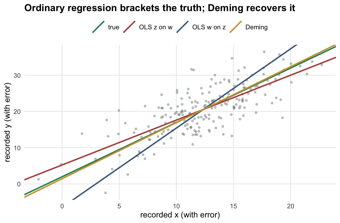
Run ordinary regression both ways. Regressing z on w treats the horizontal axis as error-free and, as before, returns an attenuated slope. Regressing w on z treats the vertical axis as error-free; inverting that fit to express it as a slope of z on w returns something too steep. The true slope is trapped between them.

f_yx  <- lm(z ~ w)                       # forward: attenuated
f_xy  <- lm(w ~ z)                       # inverse
b_fwd <- unname(coef(f_yx)[2])
b_inv <- unname(1 / coef(f_xy)[2])       # inverse fit expressed as z-on-w slope

Forward regression gives 1.239 and the inverted inverse regression gives 2.188, so the true 1.5 is bracketed: 1.239 below and 2.188 above. Neither is the answer, and picking whichever you ran first is picking a bias.

Deming regression with a known error ratio

Deming regression fits the line by accounting for error in both axes. It needs one piece of outside information: the ratio of the two error variances, \(\delta = \sigma_v^2 / \sigma_u^2\), error on y over error on x. Given \(\delta\), the slope has a closed form,

\[ \hat\beta \;=\; \frac{(s_{zz} - \delta\, s_{ww}) + \sqrt{(s_{zz} - \delta\, s_{ww})^2 + 4\,\delta\, s_{wz}^2}}{2\, s_{wz}}, \]

using the sample variances and covariance of the recorded data. In our design the error variances are 16 and 4, so \(\delta\) = 4. A jackknife supplies the standard error.

delta_true <- 4
dem <- deming(w, z, delta_true)

jk     <- sapply(seq_len(n), function(i) deming(w[-i], z[-i], delta_true)["slope"])
se_dem <- sqrt((n - 1) / n * sum((jk - mean(jk))^2))

b_dem <- unname(dem["slope"])
b_ma  <- unname(deming(w, z, 1)["slope"])
b_sma <- sign(cov(w, z)) * sd(z) / sd(w)

Deming returns a slope of 1.546 (jackknife standard error 0.101), back at the true 1.5 within noise. The line sits between the two ordinary fits, exactly where the truth is.

inv_a <- mean(z) - b_inv * mean(w)
lines <- data.frame(
  method    = factor(c("true", "OLS z on w", "OLS w on z", "Deming"),
                     levels = c("true", "OLS z on w", "OLS w on z", "Deming")),
  intercept = c(a0, coef(f_yx)[1], inv_a, unname(dem["intercept"])),
  slope     = c(b1, b_fwd, b_inv, b_dem)
)
ggplot(data.frame(w = w, z = z), aes(w, z)) +
  geom_point(alpha = 0.35, size = 1.1, colour = "#5d6b61") +
  geom_abline(data = lines, aes(intercept = intercept, slope = slope, colour = method),
              linewidth = 1.0) +
  scale_colour_manual(values = c("true" = col_true, "OLS z on w" = col_fwd,
                                 "OLS w on z" = col_inv, "Deming" = col_dem), name = NULL) +
  labs(title = "Ordinary regression brackets the truth; Deming recovers it",
       x = "w (recorded x, with error)", y = "z (recorded y, with error)") +
  theme_te

Figure 1: Recorded y against recorded x. Ordinary regression of z on w (red) is too shallow and of w on z (blue) is too steep; they bracket the true line (green). Deming regression with the correct error ratio (gold) lands on the truth.

The ratio is an assumption, not a result

Two special cases of Deming are common in ecology. Setting \(\delta\) = 1 gives the major axis, which minimises perpendicular distances and assumes the two errors are equal in size. The standardised major axis (reduced major axis) sets the slope to the ratio of standard deviations, sd(z) / sd(w), and is the usual tool for allometric scaling. Both are Deming under a particular guess at \(\delta\).

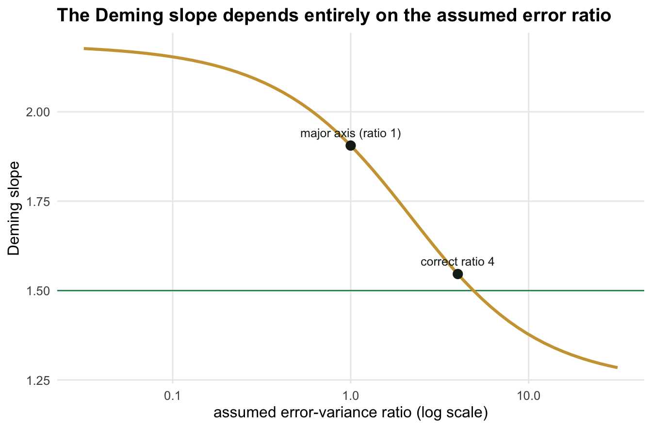
Here the errors are not equal (16 against 4), so the major axis, at 1.906, overshoots the truth by 0.406, and the standardised major axis gives 1.646. Neither is wrong as a method; each answers the question its assumption poses. The point is that the answer moves with the assumption.

Sweeping \(\delta\) makes this concrete. The Deming slope slides monotonically from the inverse regression (all error on x) to the forward regression (all error on y), passing through the major axis at \(\delta\) = 1 and hitting the truth only at the correct ratio.

delta_grid <- 10^seq(-1.5, 1.5, length.out = 60)
d2 <- data.frame(delta = delta_grid,
                 slope = sapply(delta_grid, function(d) deming(w, z, d)["slope"]))
marks <- data.frame(delta = c(1, 4),
                    slope = c(b_ma, b_dem),
                    lab   = c("major axis (ratio 1)", "correct ratio 4"))
ggplot(d2, aes(delta, slope)) +
  geom_hline(yintercept = b1, colour = col_true, linewidth = 0.5) +
  geom_line(colour = col_dem, linewidth = 1.1) +
  geom_point(data = marks, size = 3, colour = "#16241d") +
  geom_text(data = marks, aes(label = lab), vjust = -1, size = 3.3, colour = "#16241d") +
  scale_x_log10() +
  labs(title = "The Deming slope depends entirely on the assumed error ratio",
       x = "assumed error-variance ratio (log scale)", y = "Deming slope") +
  theme_te

Figure 2: Deming slope as the assumed error ratio is varied on a log scale. The horizontal line is the true slope; the estimate matches it only at the correct ratio, and drifts elsewhere. The two limits are the two ordinary regressions.

Two methods on one scale: the Bland-Altman slope

The canopy-cover comparison from the opening is usually not run as a regression at all. When two methods measure the same quantity on the same scale, the standard display is the Bland-Altman plot (Bland and Altman 1986): the difference between the methods against their mean, with limits of agreement at the mean difference plus or minus 1.96 standard deviations. A tilted cloud is then read as proportional bias and tested by regressing the difference on the mean. That reading makes the same guess as the major axis above: equal error in the two methods. Take two methods that are both unbiased (slope 1), with the error sizes of this post: method A has error sd 2, method B error sd 4, so the true ratio is the delta_true of 4 already used. The true values are drawn as in the simulation under Both axes carry error.

set.seed(20260927)
ba_n  <- 200; ba_xt <- rnorm(ba_n, mean = 12, sd = 4)
ba_a  <- ba_xt + rnorm(ba_n, 0, sd = 2)     # method A, error variance 4
ba_b  <- ba_xt + rnorm(ba_n, 0, sd = 4)     # method B, error variance 16
ba_d  <- ba_b - ba_a; ba_m <- (ba_a + ba_b) / 2
ba_co <- summary(lm(ba_d ~ ba_m))$coefficients
ba_closed <- (16 - 4) / (2 * (16 + (4 + 16) / 4))   # slope of D on M, no bias at all
ba_flat <- sqrt(1 - (16 - 4) / 16)   # true slope of B on A that makes the numerator zero
ba_loa <- mean(ba_d) + c(-1.96, 1.96) * sd(ba_d)
ba_p_lm  <- ba_co[2, 4]; ba_p_cor <- cor.test(ba_d, ba_m)$p.value; ba_p_pit <- cor.test(ba_b - 1 * ba_a, ba_b + 1 * ba_a)$p.value   # Pitman test of slope 1
stopifnot(abs(ba_p_lm - ba_p_cor) < 1e-12, abs(ba_p_lm - ba_p_pit) < 1e-12)

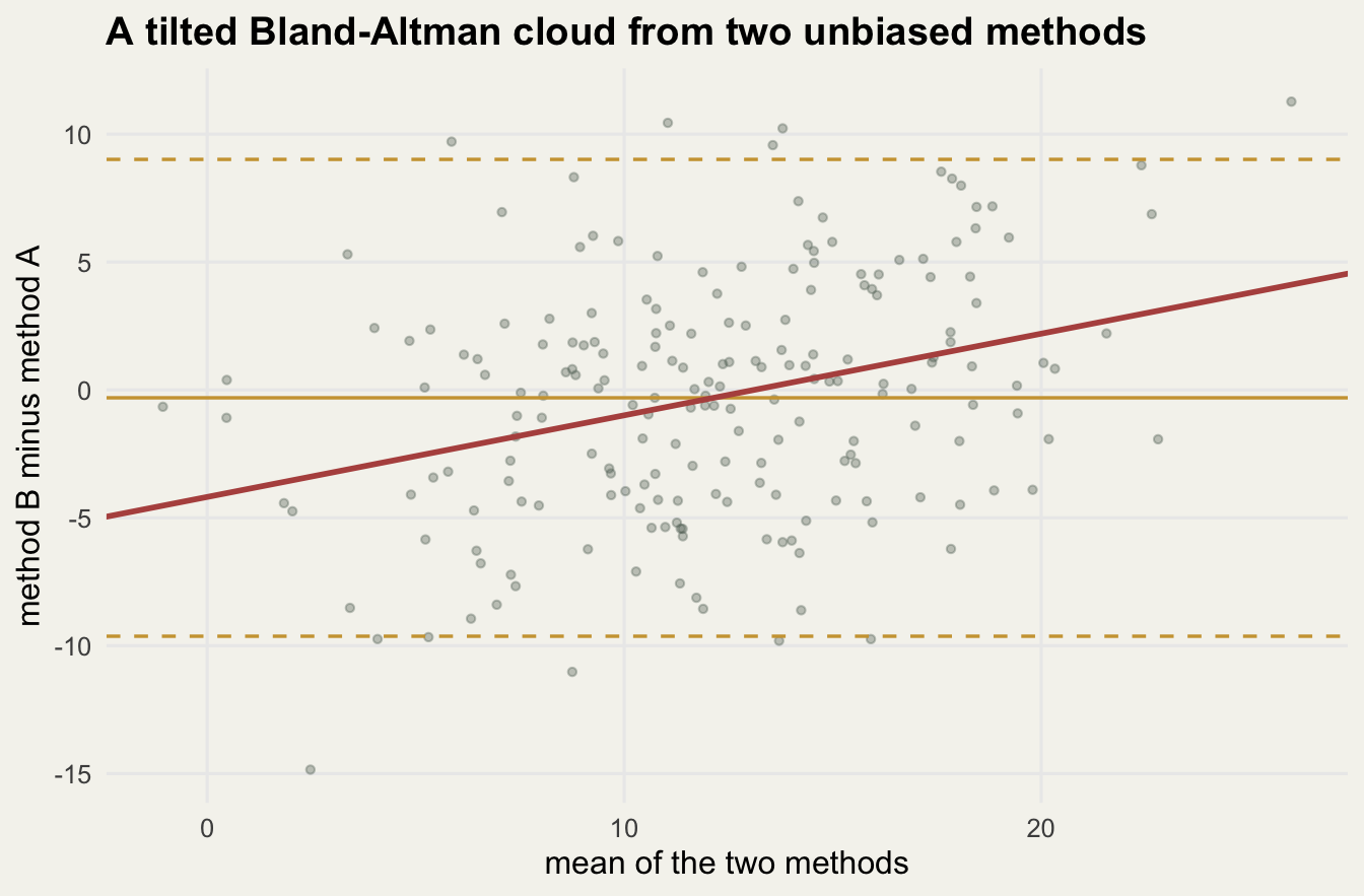
The fitted slope of difference on mean is 0.319 with p = \(4.83 \times 10^{-6}\): a textbook “proportional bias” between two methods that have none. The tilt is not noise. Neither method is biased, so the covariance of the difference and the mean is half the difference of the error variances, and the slope is that over the variance of the mean, (16 - 4) / (2 x 21) = 0.286, which this sample estimates. The test is also not what it looks like. The p value of the regression is exactly the p value of a correlation test between difference and mean, and that is the Pitman test of Testing isometry and comparing slopes with a null slope of 1, whose residual score is B - A and whose fitted score is B + A (the chunk checks all three agree). A Pitman test of slope 1 is a test that the readings of the two methods have equal variance, which for two unbiased methods means equal error variance, and here the error variances are 4 and 16. The limits of agreement are not affected: they run from -9.6 to 9.0 and describe how far apart two readings can be, which is what they are for.

ggplot(data.frame(m = ba_m, d = ba_d), aes(m, d)) +
  geom_point(alpha = 0.35, size = 1.1, colour = "#5d6b61") +
  geom_hline(yintercept = mean(ba_d), colour = col_dem, linewidth = 0.6) +
  geom_hline(yintercept = ba_loa, colour = col_dem, linewidth = 0.6, linetype = "dashed") +
  geom_abline(intercept = ba_co[1, 1], slope = ba_co[2, 1], colour = col_fwd, linewidth = 1.0) +
  labs(title = "A tilted Bland-Altman cloud from two unbiased methods",
       x = "mean of the two methods", y = "method B minus method A") +
  theme_te

Figure 3: Bland-Altman plot of two unbiased methods whose errors differ (sd 2 and 4). The regression of difference on mean (red) rises although neither method is biased; the dashed lines are the limits of agreement.

How often does the test raise the flag, and what should replace it? The chunk below repeats the design 1000 times at three sample sizes and scores five tests at the 5 per cent level. After the Bland-Altman test come four Deming tests of the slope of B on A against 1 with a bootstrap standard error (199 resamples of units, normal reference): the major axis (ratio 1), Deming with the true ratio, and Deming with a ratio measured from duplicates, 20 units read twice by each method, first held fixed in the bootstrap and then re-estimated in every resample by resampling the duplicate pairs too.

set.seed(4527); ba_reps <- 1000; ba_boot <- 199; ba_ndup <- 20
ba_dem <- function(sxx, syy, sxy, d) ((syy - d*sxx) + sqrt((syy - d*sxx)^2 + 4*d*sxy^2)) / (2*sxy)
ba_one <- function(n) {
  xt_i <- rnorm(n, 12, 4); a <- xt_i + rnorm(n, 0, 2); b <- xt_i + rnorm(n, 0, 4)
  p_ba <- summary(lm(I(b - a) ~ I((a + b) / 2)))$coefficients[2, 4]
  dup_a <- rnorm(ba_ndup, 0, 2) - rnorm(ba_ndup, 0, 2); dup_b <- rnorm(ba_ndup, 0, 4) - rnorm(ba_ndup, 0, 4)
  d_hat <- sum(dup_b^2) / sum(dup_a^2)
  ui <- matrix(sample.int(n, n * ba_boot, replace = TRUE), n); di <- matrix(sample.int(ba_ndup, ba_ndup * ba_boot, replace = TRUE), ba_ndup)
  ab <- matrix(a[ui], n); bb <- matrix(b[ui], n)
  sxx <- apply(ab, 2, var); syy <- apply(bb, 2, var)
  sxy <- (colSums(ab * bb) - n * colMeans(ab) * colMeans(bb)) / (n - 1)
  d_boot <- colSums(matrix(dup_b[di], ba_ndup)^2) / colSums(matrix(dup_a[di], ba_ndup)^2)
  est <- sapply(c(ma = 1, known = delta_true, fixed = d_hat), function(r) deming(a, b, r)[["slope"]])
  se  <- sapply(list(ma = 1, known = delta_true, fixed = d_hat, resampled = d_boot),
                function(r) sd(ba_dem(sxx, syy, sxy, r)))
  est <- c(est, resampled = est[["fixed"]])
  c(bland_altman = p_ba < 0.05, abs(est - 1) / se > qnorm(0.975), ma_slope = est[["ma"]],
    ma_same = (est[["ma"]] > 1) == (var(b) > var(a)))
}
ba_ns  <- c(30, 100, 400); ba_res <- sapply(ba_ns, function(n) rowMeans(replicate(ba_reps, ba_one(n))))
ba_pow <- pnorm(atanh(6 / sqrt(20 * 21)) * sqrt(ba_ns - 3) - qnorm(0.975))   # Fisher z power
ba_mcse <- sqrt(c(0.05 * 0.95, 0.25) / ba_reps); ba_f3 <- function(row) paste(sprintf("%.3f", ba_res[row, ]), collapse = ", ")
ba_ma_pop <- (12 + sqrt(12^2 + 4 * 16^2)) / (2 * 16)   # major axis from population moments
stopifnot(all(ba_res["ma_same", ] == 1))                # MA slope > 1 exactly when var(B) > var(A)

At n = 30, 100 and 400 the Bland-Altman test flags proportional bias in a share 0.361, 0.840, 1.000 of data sets. That is no simulation finding: it is the power of the correlation test against the population correlation 6 / sqrt(20 x 21), which the Fisher z approximation puts at 0.347, 0.844, 1.000, and the simulation reproduces it. The major axis makes the same equal-error guess and fails the same way, flagging 0.129, 0.718, 1.000 because its slope settles at 1.443 rather than 1 (mean over data sets 1.509, 1.458, 1.452). Its slope exceeds 1 exactly when the readings of B vary more than those of A (the chunk checks this in every data set), so it tests the same hypothesis as the Bland-Altman slope; its lower rate at small n comes from the weaker bootstrap z test, not from a smaller problem. Deming with the true ratio, the tool this post already has, holds its level at n = 100 and 400 (0.055 and 0.056) and runs above it at n = 30 (0.073), where a bootstrap z test on 30 units is itself on thin ground. (Monte Carlo standard error: 0.007 for a rate near 0.05, 0.016 at most.)

The catch is that nobody knows the true ratio; it has to be measured, and a measured ratio is an estimate. With the ratio from 20 duplicate pairs held fixed, the Deming test rejects 0.081, 0.103, 0.246: at n = 30 hardly more than the true-ratio row, then too often, and increasingly so as n grows. The error in the ratio is set by the number of duplicate pairs, not by n, so as the units pin the slope down more tightly, the part of the uncertainty the test ignores becomes a larger share of the whole. Resampling the duplicate pairs together with the units carries that uncertainty and brings the rate back to 0.065, 0.044, 0.054, in line with the true-ratio row. It is the point Checking a measurement-error correction makes about reliability, and the one How long a calibration overlap do you need? takes from Bland and Altman: the agreement between two methods is itself estimated. Two limits bound this. A Bland-Altman slope cannot tell unequal precision from a true proportional bias: with error sds sA and sB (here 2 and 4), a true slope beta of B on A and true-value sd sT, the numerator of the slope becomes sB^2 - sA^2 + (beta^2 - 1) sT^2, and the two terms simply add, so a tilted plot is compatible with either or both. They can also cancel: with the error sizes here, a true slope of 0.5 gives a flat plot (16 - 4 + (0.25 - 1) x 16 = 0), so a level cloud is no evidence against proportional bias either. Separating them needs the error variances, which means repeat readings by both methods, the same boundary as the end of this post. And the rates for the fixed ratio belong to 20 pairs per method and this design.

What to take away

With error on both axes, ordinary regression brackets the truth but never delivers it, and which side you land on is decided by which variable you happen to call the response. Deming regression removes that arbitrariness once you supply the ratio of error variances. Everything then rests on that ratio: the major axis assumes it is one, the standardised major axis assumes error scales with spread, and a Deming fit assumes whatever value you feed it.

So the honest boundary is sharp. If replicate measurements or instrument specifications pin the error variances, Deming is a clean fix. If the ratio is unknown, the model is not identified from the recorded data alone; you are choosing a slope by choosing an assumption, and the choice should be stated rather than buried.

Where to go next

When the model is more elaborate than a straight line, or when the error affects the predictor through a nonlinear term, the closed-form corrections stop applying. A simulation-based method sidesteps that by adding error on purpose and extrapolating back. The closing post then returns to the question every correction here quietly assumed: where the error variance actually comes from.

References

• Deming 1943 Statistical Adjustment of Data, ISBN 978-0-486-64685-5
• Warton, Wright, Falster, Westoby 2006 Biological Reviews 81(2):259-291 (10.1017/S1464793106007007)
• Carroll, Ruppert, Stefanski, Crainiceanu 2006 Measurement Error in Nonlinear Models, 2nd ed, ISBN 978-1-58488-633-4
• Bland, Altman 1986 The Lancet 327(8476):307-310 (10.1016/S0140-6736(86)90837-8)
• Linnet 1993 Clinical Chemistry 39(3):424-432 (10.1093/clinchem/39.3.424)

Related tutorials

• Measurement error and regression dilution
• Correcting measurement error with SIMEX
• Checking a measurement-error correction
• How long a calibration overlap do you need?

Reproducibility

• Code last run: 2026-09-30
• R version 4.5.3 (2026-03-11), aarch64-apple-darwin20
• Packages: dplyr 1.2.1, ggplot2 4.0.3, tidyr 1.3.2