---
title: "Measurement error and regression dilution"
description: "Error in an environmental predictor biases regression slopes towards zero. See how the reliability ratio attenuates estimates in R, and how to correct them."
date: "2026-05-27 12:00"
categories: ["R", "ecology tutorial", "regression", "measurement error", "simulation"]
image: thumbnail.png
image-alt: "The same responses plotted against a true predictor and a noisy recorded one, the wider cloud giving a visibly shallower fitted line."
---
Field ecology runs on predictors that are measured, not known. Soil moisture read from a probe, canopy cover scored by eye, a remotely sensed temperature, a body size taken with callipers: each carries error. It is tempting to treat the recorded value as the truth and fit the usual regression. The recorded value is not the truth, and the regression pays for the difference in a specific, predictable way. The slope shrinks towards zero. A real effect looks weaker than it is, and a borderline effect can vanish.
This post shows the mechanism with a small simulation, quantifies it with the reliability ratio, and corrects it when the size of the error is known. It also draws the contrast that trips people up: error in the *response* behaves nothing like error in a *predictor*.
```{r}
#| label: setup
#| code-fold: true
#| code-summary: "Setup: packages, colours and plot theme"
#| results: hide
#| message: false
#| warning: false
suppressMessages({library(ggplot2); library(dplyr); library(tidyr)})

theme_te <- theme_minimal(base_size = 12) +
  theme(
        plot.background  = element_rect(fill = "#f5f4ee", colour = NA),
        panel.background = element_rect(fill = "#f5f4ee", colour = NA),
        panel.grid.minor = element_blank(),
        plot.title = element_text(face = "bold"),
        legend.position = "top")
col_true <- "#2f8f63"; col_obs <- "#b5534e"; col_corr <- "#cda23f"
```
## A predictor measured with error
The set-up is deliberately plain. A response depends linearly on a true predictor `x`, with intercept `1` and slope `2`. We never see `x`; we see `w`, which is `x` plus independent, mean-zero measurement error. This is *classical* measurement error: the error does not depend on `x`, on the response, or on anything else.
```{r}
#| label: simulate
set.seed(4127)
n   <- 300
b0  <- 1; b1 <- 2
sdx <- 3            # spread of the true predictor: var_x = 9
sde <- 2            # residual spread
sdu <- 3            # measurement-error spread: var_u = 9

x <- rnorm(n, mean = 10, sd = sdx)
y <- b0 + b1 * x + rnorm(n, 0, sde)
w <- x + rnorm(n, 0, sdu)          # what we actually record

fit_true  <- lm(y ~ x)             # unavailable in practice
fit_naive <- lm(y ~ w)             # what everyone fits
```
```{r}
#| label: naive-numbers
#| code-fold: true
#| code-summary: "Code for the numbers quoted in the text"
#| results: hide
#| message: false
#| warning: false
b_true  <- unname(coef(fit_true)[2]);  se_true  <- summary(fit_true)$coef[2, 2]
b_naive <- unname(coef(fit_naive)[2]); se_naive <- summary(fit_naive)$coef[2, 2]
lambda  <- sdx^2 / (sdx^2 + sdu^2)
```
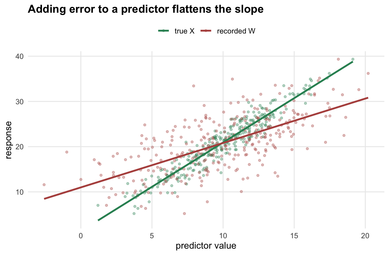
Fitting against the true `x` recovers the slope: `r round(b_true, 3)`. Fitting against the recorded `w` gives `r round(b_naive, 3)`, roughly half of the truth. That halving is not bad luck. With classical error, the naive slope estimates the true slope multiplied by the **reliability ratio**
$$
\lambda = \frac{\sigma_x^2}{\sigma_x^2 + \sigma_u^2},
$$
the share of the recorded variance that is real signal rather than error. Here `x` and the error have equal variance (`9` and `9`), so $\lambda$ = `r round(lambda, 2)` and the expected naive slope is $\lambda\,\beta_1$ = `r round(lambda * b1, 2)`. The simulated naive slope, `r round(b_naive, 3)`, sits right on it.
The picture is the whole story. Adding error stretches the cloud sideways without moving it up or down, so a line through the wider cloud has to be shallower.
```{r}
#| label: fig-attenuation
#| fig-cap: "The same responses plotted against the true predictor (green) and against the error-prone recorded predictor (red). Horizontal spreading flattens the fitted line."
#| fig-alt: "Scatter plot of response against predictor value. Green points against the true predictor form a tight steep band with a steep fitted line. Red points against the recorded predictor are spread wider horizontally and their fitted line is visibly shallower, passing through the same centre."
#| fig-width: 7
#| fig-height: 4.6
d1 <- bind_rows(
  data.frame(pred = x, y = y, kind = "true X"),
  data.frame(pred = w, y = y, kind = "recorded W")
)
d1$kind <- factor(d1$kind, levels = c("true X", "recorded W"))

ggplot(d1, aes(pred, y, colour = kind)) +
  geom_point(alpha = 0.35, size = 1.1) +
  geom_smooth(method = "lm", formula = y ~ x, se = FALSE, linewidth = 1.1) +
  scale_colour_manual(values = c("true X" = col_true, "recorded W" = col_obs),
                      name = NULL) +
  labs(title = "Adding error to a predictor flattens the slope",
       x = "predictor value", y = "response") +
  theme_te
```
## Correcting when the error variance is known
Attenuation is reversible if you know how much error you added. The method-of-moments correction divides the naive slope by an estimate of the reliability ratio. You never see $\sigma_x^2$ directly, but you do see the variance of `w`, and $\sigma_x^2 = \operatorname{var}(w) - \sigma_u^2$. So with $\sigma_u^2$ in hand (from an instrument specification, or from replicate measurements, the subject of a later post) the reliability is estimated from the recorded data alone.
```{r}
#| label: correct
var_u      <- sdu^2                       # assumed known
lambda_hat <- (var(w) - var_u) / var(w)   # reliability from the recorded data
b_corr     <- b_naive / lambda_hat        # attenuation-corrected slope
se_corr    <- se_naive / lambda_hat       # uncertainty grows in step
```
The estimated reliability is `r round(lambda_hat, 3)`, close to the true `r round(lambda, 2)`. Dividing through gives a corrected slope of `r round(b_corr, 3)`, back at the true value of `2`. The correction is not free. The standard error rises from `r round(se_naive, 3)` to `r round(se_corr, 3)`, because dividing by a number below one inflates the spread as well as the estimate. That trade is the honest cost of the fix: you recover the location by paying in precision.
## The attenuation curve
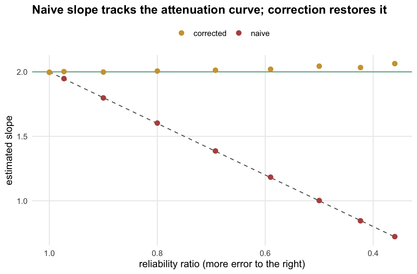
Sweeping the error variance shows the effect in one line. For each level of measurement error we simulate many datasets, record the mean naive slope, and record the mean corrected slope. The naive slopes fall along the theoretical curve $\beta_1\lambda$; the corrected slopes stay flat at the truth.
```{r}
#| label: sweep
set.seed(2024)
sdu_grid <- seq(0, 4, by = 0.5)
reps     <- 400
naive_s <- corr_s <- numeric(length(sdu_grid))
for (i in seq_along(sdu_grid)) {
  su <- sdu_grid[i]
  ns <- cs <- numeric(reps)
  for (r in seq_len(reps)) {
    xx <- rnorm(n, 10, sdx)
    yy <- b0 + b1 * xx + rnorm(n, 0, sde)
    ww <- xx + rnorm(n, 0, su)
    bn <- coef(lm(yy ~ ww))[2]
    lh <- (var(ww) - su^2) / var(ww)
    ns[r] <- bn; cs[r] <- bn / lh
  }
  naive_s[i] <- mean(ns); corr_s[i] <- mean(cs)
}
lam_grid <- sdx^2 / (sdx^2 + sdu_grid^2)
```
```{r}
#| label: sweep-numbers
#| include: false
max_dev_corr <- max(abs(corr_s - b1))
max_dev_naive <- max(abs(naive_s - b1 * lam_grid))
```
```{r}
#| label: fig-curve
#| fig-cap: "Mean naive slope (red) and mean corrected slope (gold) across levels of measurement error. Dashed line is the theoretical attenuation curve; the horizontal line marks the true slope of 2."
#| fig-alt: "Estimated slope against reliability ratio, with more measurement error to the right. Red points fall steadily below the true slope and lie on a dashed theoretical curve. Gold points stay flat along the horizontal line at slope 2 across the whole range."
#| fig-width: 7
#| fig-height: 4.6
d2 <- data.frame(lambda = lam_grid, naive = naive_s, corrected = corr_s,
                 theory = b1 * lam_grid) |>
  pivot_longer(c(naive, corrected), names_to = "estimator", values_to = "slope")

ggplot(d2, aes(lambda)) +
  geom_line(aes(y = theory), linetype = "dashed", colour = "#5d6b61") +
  geom_hline(yintercept = b1, colour = col_true, linewidth = 0.4) +
  geom_point(aes(y = slope, colour = estimator), size = 2.4) +
  scale_colour_manual(values = c(naive = col_obs, corrected = col_corr), name = NULL) +
  scale_x_reverse() +
  labs(title = "Naive slope tracks the attenuation curve; correction restores it",
       x = "reliability ratio (more error to the right)", y = "estimated slope") +
  theme_te
```
Across the grid the naive slope never strays more than `r round(max_dev_naive, 3)` from the theoretical curve, and the corrected slope never strays more than `r round(max_dev_corr, 3)` from the truth. One caution the figure hides: as reliability falls towards zero the correction divides by an ever smaller, ever noisier number, so at very low reliability the corrected estimate becomes erratic. Correcting a badly measured predictor is possible in principle and unstable in practice.
## Error in the response is a different animal
The result above is specific to error in a *predictor*. Put the same error on the *response* instead and the slope is untouched. Additive mean-zero noise on `y` folds into the residual term, which regression already expects. It widens the standard error and lowers the fit, but it does not tilt the line.
```{r}
#| label: response-error
set.seed(9931)
y_noisy <- y + rnorm(n, 0, 4)      # error added to the response, not the predictor
fit_yv  <- lm(y_noisy ~ x)
```
```{r}
#| label: response-numbers
#| include: false
b_yv <- unname(coef(fit_yv)[2]); se_yv <- summary(fit_yv)$coef[2, 2]
r2_a <- summary(fit_true)$r.squared
r2_b <- summary(fit_yv)$r.squared
```
With heavy error on the response the slope is `r round(b_yv, 3)`, still at the truth, while its standard error widens from `r round(se_true, 3)` to `r round(se_yv, 3)` and the R-squared drops from `r round(r2_a, 3)` to `r round(r2_b, 3)`. So the direction to check matters. A noisy response costs you precision; a noisy predictor costs you the estimate.
## What to take away
Classical measurement error in a predictor multiplies the slope by the reliability ratio, pulling it towards zero, and no amount of extra data removes the bias: more sampling of a mismeasured quantity sharpens a biased target. The fix needs external knowledge of the error, which is exactly the assumption to be honest about. If $\sigma_u^2$ is known you can divide it out, trading bias for variance. If it is not, you cannot recover it from the recorded data alone, and you fall back on replicate measurements or a validation subsample to estimate reliability.
Two extensions are worth flagging. With several predictors, error in one does not stay in its own lane: it can bias every coefficient in the model, including well-measured ones, so a single noisy covariate contaminates the whole fit. And a slope of exactly zero is the one value classical error leaves alone, which is a useful sanity check: attenuation cannot manufacture an effect, only weaken a real one.
## Where to go next
The next step is the harder case where *both* variables carry error, so ordinary regression no longer brackets the truth from a known side. After that, a simulation-based correction handles messier models where a neat variance formula is not available, and a closing post covers how you actually get the error variance in the first place.
## References
- Spearman 1904 American Journal of Psychology 15(1):72-101 (10.2307/1412159)
- Frost, Thompson 2000 Journal of the Royal Statistical Society A 163(2):173-189 (10.1111/1467-985X.00164)
- Carroll, Ruppert, Stefanski, Crainiceanu 2006 Measurement Error in Nonlinear Models, 2nd ed, ISBN 978-1-58488-633-4
- Fuller 1987 Measurement Error Models, ISBN 978-0-471-86187-4
## Related tutorials
- [Size measurement error in an IPM](../size-measurement-error-in-an-ipm/)
- [Correcting measurement error with SIMEX](../simex-measurement-error-correction/)
- [Additive or compensatory harvest mortality](../additive-or-compensatory-harvest/)
- [Dichotomising a continuous confounder](../dichotomising-a-continuous-predictor/)