---
title: "Correcting measurement error with SIMEX"
description: "SIMEX corrects measurement error by simulation: add known error, watch the estimate degrade, then extrapolate back to none. A from-scratch tutorial in R."
date: "2026-05-27 14:00"
categories: ["R", "ecology tutorial", "regression", "measurement error", "simulation"]
image: thumbnail.png
image-alt: "Slope estimates falling as measurement error is added, with the fitted curve extrapolated back into a shaded band towards the true slope."
---
The moment correction in the first post divided the attenuated slope by the reliability ratio. That works for a straight line. The moment it turns nonlinear, or the error enters through a squared term or a link function, the tidy formula stops applying and there is no obvious quantity to divide by. SIMEX, simulation-extrapolation, gets around this by not needing a formula at all. It learns how the estimate reacts to measurement error by *adding more of it*, then extrapolates the trend back to the hypothetical case of no error.
The idea sounds circular and is not. This post builds SIMEX by hand on a linear model, where a closed-form correction exists to check it against, so the mechanics are visible before you trust them on a model where no check is available.
```{r}
#| label: setup
#| code-fold: true
#| code-summary: "Setup: packages, colours and plot theme"
#| results: hide
#| message: false
#| warning: false
suppressMessages({library(ggplot2); library(dplyr)})
theme_te <- theme_minimal(base_size = 12) +
  theme(
        plot.background  = element_rect(fill = "#f5f4ee", colour = NA),
        panel.background = element_rect(fill = "#f5f4ee", colour = NA),
        panel.grid.minor = element_blank(),
        plot.title = element_text(face = "bold"), legend.position = "top")
col_pt <- "#275139"; col_q <- "#b5534e"; col_r <- "#cda23f"; col_true <- "#2f8f63"
```
## The two ideas
SIMEX rests on two observations. First, measurement error is something you can add, and its effect on an estimate is smooth: put more error on the predictor and the slope attenuates further, in a regular way. Second, if you can trace that regular relationship between the amount of error and the estimate, you can read off where it heads as the error goes to zero, even though zero error is unreachable in the recorded data.
Concretely: the recorded predictor already carries error of a known variance. Add extra simulated error of variance $\lambda\,\sigma_u^2$ for a range of $\lambda \ge 0$. Refit at each level, and the total error is $(1 + \lambda)\sigma_u^2$. The recorded data itself is the $\lambda = 0$ point, with total error $\sigma_u^2$. The value you actually want, no measurement error, sits at $\lambda = -1$, where total error is zero. You cannot simulate negative error, but you can fit a curve to the $\lambda \ge 0$ points and extrapolate it to $\lambda = -1$.
## The simulation step
The set-up matches the first post so the answer is known: slope `2`, a predictor with variance `9`, and measurement error of variance `4`, giving a reliability of about `0.69`.
```{r}
#| label: simulate
set.seed(78)
n     <- 300
b0    <- 1; b1 <- 2
sdx   <- 3; sde <- 2
sdu   <- 2                       # measurement-error sd; variance 4 assumed known
var_u <- sdu^2

x <- rnorm(n, 10, sdx)
y <- b0 + b1 * x + rnorm(n, 0, sde)
w <- x + rnorm(n, 0, sdu)
```
For each level of added error, add fresh noise to `w`, refit, and average the slope over many draws to damp the simulation noise.
```{r}
#| label: simex-loop
lambda_grid <- seq(0, 2, by = 0.25)
B           <- 200
beta_lambda <- numeric(length(lambda_grid))

set.seed(99)
for (i in seq_along(lambda_grid)) {
  la <- lambda_grid[i]
  bb <- numeric(B)
  for (b in seq_len(B)) {
    w_star <- w + rnorm(n, 0, sqrt(la * var_u))   # extra error, variance la * var_u
    bb[b]  <- coef(lm(y ~ w_star))[2]
  }
  beta_lambda[i] <- mean(bb)
}
```
```{r}
#| label: simex-numbers
#| code-fold: true
#| code-summary: "Code for the numbers quoted in the text"
#| results: hide
#| message: false
#| warning: false
b_naive <- beta_lambda[1]
```
The first grid point, at zero added error, is just the naive slope: `r round(b_naive, 3)`. From there the slope falls steadily as error piles on, reaching `r round(beta_lambda[length(beta_lambda)], 3)` at the far end. That downward march is the signal SIMEX extrapolates.
## The extrapolation step
Fit a curve to the grid and evaluate it at $\lambda = -1$. The standard default is a quadratic in $\lambda$. It has no special justification beyond being a flexible local approximation, which is the honest way to describe it.
```{r}
#| label: extrapolate-quad
ext_q   <- lm(beta_lambda ~ lambda_grid + I(lambda_grid^2))
simex_q <- unname(predict(ext_q, newdata = data.frame(lambda_grid = -1)))
```
```{r}
#| label: quad-number
#| include: false
```
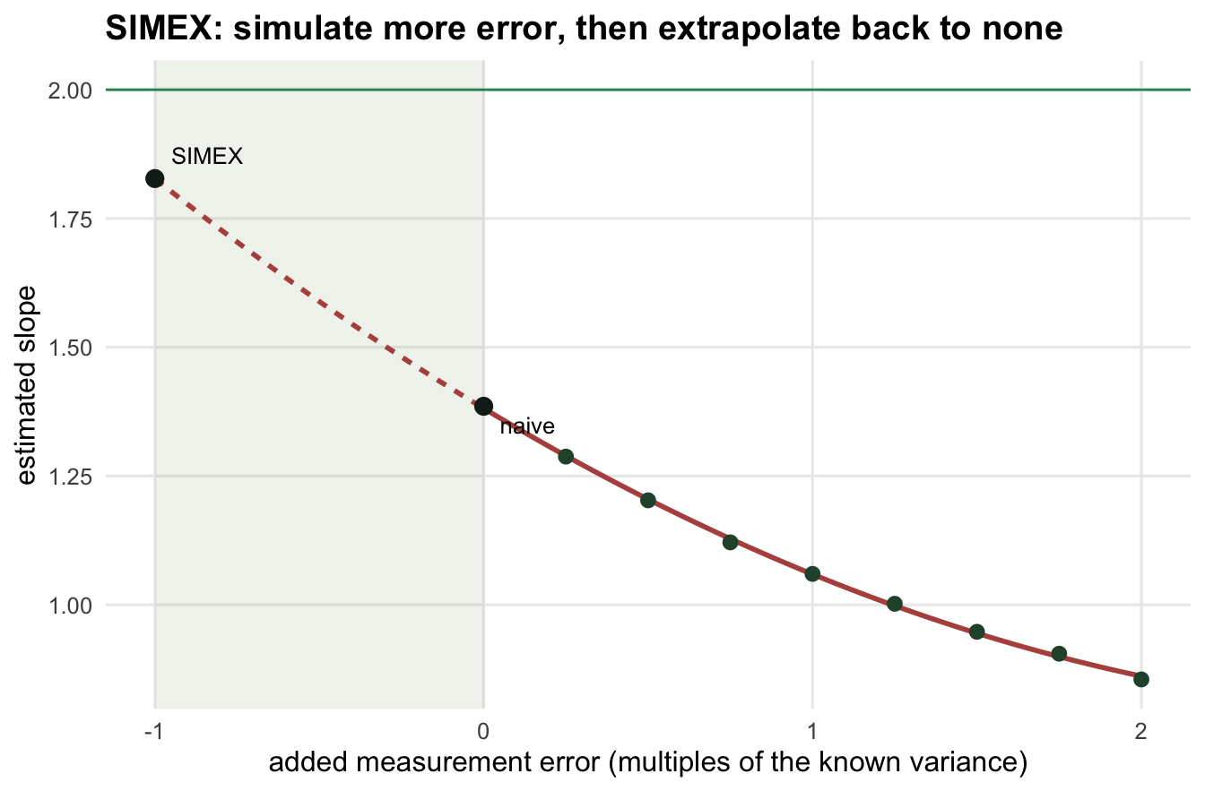
The quadratic extrapolant reaches `r round(simex_q, 3)` at $\lambda = -1$, up from the naive `r round(b_naive, 3)` and most of the way back to the true `2`. The diagram is the method in one glance: real estimates on the right, extrapolated correction on the left, in a region where no data exist.
```{r}
#| label: fig-simex
#| fig-cap: "The SIMEX diagram. Green points are slopes at increasing added error; the red curve is the quadratic extrapolant. The naive estimate is at zero added error; the SIMEX estimate is the curve extended into the shaded no-data region at minus one, where total error would be zero. The horizontal line is the true slope."
#| fig-alt: "Estimated slope against added measurement error. Green points descend from left to right. A red fitted curve passes through them and is extended as a dashed line leftwards into a shaded band, rising back up towards a horizontal true-slope line and ending at a black point labelled SIMEX at minus one on the axis."
#| fig-width: 7
#| fig-height: 4.6
grid_plot <- seq(-1, 2, length.out = 200)
dcur <- data.frame(lambda_add = grid_plot,
                   slope = predict(ext_q, data.frame(lambda_grid = grid_plot)))
dpts <- data.frame(lambda_add = lambda_grid, slope = beta_lambda)

ggplot() +
  annotate("rect", xmin = -1, xmax = 0, ymin = -Inf, ymax = Inf,
           fill = "#93a87f", alpha = 0.14) +
  geom_hline(yintercept = b1, colour = col_true, linewidth = 0.5) +
  geom_line(data = subset(dcur, lambda_add >= 0), aes(lambda_add, slope),
            colour = col_q, linewidth = 1.0) +
  geom_line(data = subset(dcur, lambda_add <= 0), aes(lambda_add, slope),
            colour = col_q, linewidth = 1.0, linetype = "22") +
  geom_point(data = dpts, aes(lambda_add, slope), colour = col_pt, size = 2.4) +
  annotate("point", x = 0, y = b_naive, colour = "#16241d", size = 3) +
  annotate("point", x = -1, y = simex_q, colour = "#16241d", size = 3) +
  annotate("text", x = 0.05, y = b_naive, label = "naive", hjust = 0, vjust = 1.6, size = 3.4) +
  annotate("text", x = -0.95, y = simex_q, label = "SIMEX", hjust = 0, vjust = -0.9, size = 3.4) +
  labs(title = "SIMEX: simulate more error, then extrapolate back to none",
       x = "added measurement error (multiples of the known variance)",
       y = "estimated slope") +
  theme_te
```
## Checking it, and the choice it hides
For a linear model the correction can be checked two ways. The moment correction from the first post divides the naive slope by the reliability, and there is an extrapolant that is exactly right for this model: the rational-linear form $\beta(\lambda) = (\gamma_0 + \gamma_1\lambda)/(\gamma_2 + \lambda)$, because attenuation really is a hyperbola in $\lambda$.
```{r}
#| label: extrapolate-rational
# beta(lambda) = (g0 + g1*lambda)/(g2 + lambda) is linear in the parameters once the
# denominator is cleared: beta*lambda = g0 + g1*lambda - g2*beta. That linear fit supplies
# starting values near the optimum, and the port algorithm handles the shallow,
# ill-conditioned valley (the grid points are nearly straight in lambda over 0 to 2).
lin_start <- lm(I(beta_lambda * lambda_grid) ~ lambda_grid + beta_lambda)
ext_r   <- nls(beta_lambda ~ (g0 + g1 * lambda_grid) / (g2 + lambda_grid),
               start = list(g0 =  unname(coef(lin_start)[1]),
                            g1 =  unname(coef(lin_start)[2]),
                            g2 = -unname(coef(lin_start)[3])),
               algorithm = "port")
cf      <- coef(ext_r)
simex_r <- unname((cf["g0"] + cf["g1"] * (-1)) / (cf["g2"] + (-1)))

lam_hat  <- (var(w) - var_u) / var(w)
b_moment <- unname(coef(lm(y ~ w))[2] / lam_hat)
```
```{r}
#| label: check-numbers
#| include: false
```
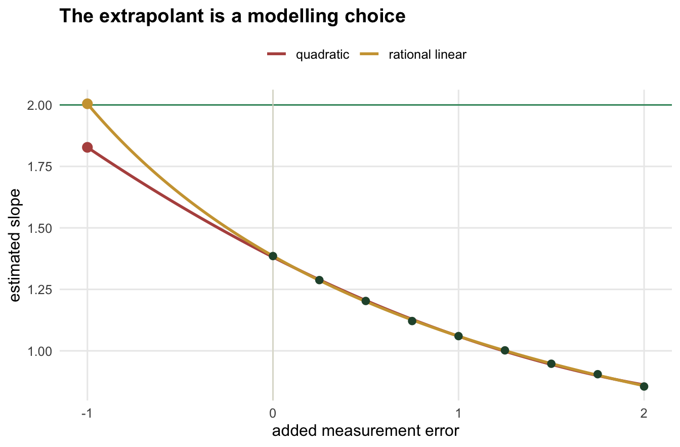
The rational-linear extrapolant gives `r round(simex_r, 3)`, effectively identical to the moment correction, `r round(b_moment, 3)`, and on the true value of `2`. The quadratic, at `r round(simex_q, 3)`, undershoots a little. The two extrapolants fit the same grid points and part company only where it matters, out in the extrapolation.
```{r}
#| label: fig-extrapolant
#| fig-cap: "The same grid points fitted with a quadratic (red) and a rational-linear (gold) extrapolant. They agree over the data and diverge in the extrapolation to no error: the rational-linear form is exact for a linear model, the quadratic is an approximation."
#| fig-alt: "Two fitted curves through the same green points. To the right of zero the red and gold curves lie almost on top of each other. To the left, extrapolating towards minus one, the gold rational-linear curve rises to the true-slope line while the red quadratic curve rises more slowly and ends at about 1.83, below the true-slope line, so the two curves end at separate points."
#| fig-width: 7
#| fig-height: 4.6
pr <- (cf["g0"] + cf["g1"] * grid_plot) / (cf["g2"] + grid_plot)
d2 <- rbind(
  data.frame(lambda_add = grid_plot, slope = dcur$slope, extrapolant = "quadratic"),
  data.frame(lambda_add = grid_plot, slope = pr,        extrapolant = "rational linear"))

ggplot() +
  geom_hline(yintercept = b1, colour = col_true, linewidth = 0.5) +
  geom_vline(xintercept = 0, colour = "#dad9ca", linewidth = 0.4) +
  geom_line(data = d2, aes(lambda_add, slope, colour = extrapolant), linewidth = 1.0) +
  geom_point(data = dpts, aes(lambda_add, slope), colour = col_pt, size = 2.2) +
  annotate("point", x = -1, y = simex_q, colour = col_q, size = 3) +
  annotate("point", x = -1, y = simex_r, colour = col_r, size = 3) +
  scale_colour_manual(values = c("quadratic" = col_q, "rational linear" = col_r), name = NULL) +
  labs(title = "The extrapolant is a modelling choice",
       x = "added measurement error", y = "estimated slope") +
  theme_te
```
## What to take away
SIMEX corrects measurement error without a bias formula. It adds known error, records how the estimate slides, and extrapolates that slide back to the no-error case. Because the only model-specific step is refitting, the same recipe carries to logistic regression, a generalised additive model, or any fit where writing down the attenuation by hand would be painful. On the linear model here it reproduces the closed-form correction, which is the reassurance that the extrapolation is doing something sensible rather than something convenient.
Two honesties travel with it. It still needs the measurement-error variance as an input: the whole scheme is calibrated in multiples of $\sigma_u^2$, so without that number there is nothing to add or extrapolate. And the extrapolant is a genuine choice, not a detail. The quadratic default is convenient and approximate; a different functional form gives a different answer at $\lambda = -1$, and the further you extrapolate the more the choice bites. Report which extrapolant you used, and treat a correction that swings wildly between forms as a warning rather than a result. The final post takes up the input every method here has leaned on: how you actually measure the measurement error.
## Where to go next
Every correction across these posts, dividing by the reliability, choosing an error ratio, calibrating SIMEX in multiples of the error variance, took the size of the measurement error as given. The last post is about earning that number: estimating reliability from replicate measurements, checking whether error is even worth correcting, and running a sensitivity analysis when the error variance is a guess rather than a measurement.
## References
- Cook, Stefanski 1994 Journal of the American Statistical Association 89(428):1314-1328 (10.1080/01621459.1994.10476871)
- Stefanski, Cook 1995 Journal of the American Statistical Association 90(432):1247-1256 (10.1080/01621459.1995.10476629)
- Carroll, Ruppert, Stefanski, Crainiceanu 2006 Measurement Error in Nonlinear Models, 2nd ed, ISBN 978-1-58488-633-4
- Lederer, Kuchenhoff 2006 R News 6(4):26-31 (ISSN 1609-3631)
## Related tutorials
- [Measurement error and regression dilution](../measurement-error-regression-dilution/)
- [Errors-in-variables and Deming regression](../errors-in-variables-deming-regression/)
- [Checking a measurement-error correction](../checking-measurement-error-corrections/)
- [Power analysis by simulation](../power-analysis-by-simulation/)