set.seed(42)
n <- 80
elevation   <- runif(n, 200, 2000)                          # metres
temperature <- 24 - 0.0065 * elevation + rnorm(n, 0, 0.8)    # lapse rate
precip      <- 800 + 0.15 * elevation + rnorm(n, 0, 180)     # mild elevation link
carbon      <- 6 + 0.9 * temperature + rnorm(n, 0, 3)        # responds to temperature only
dat <- data.frame(carbon, temperature, elevation, precip)Collinearity and VIF in ecological regression
R
regression
diagnostics
ecology tutorial
Correlated predictors inflate standard errors and destabilise coefficients in ecological regression. Compute the VIF by hand in R, read it, and act on it.
Ecological predictors rarely arrive independent of one another. Elevation, temperature and precipitation move together; canopy cover tracks soil moisture; latitude stands in for half a dozen climate gradients at once. When two or more predictors in a regression carry overlapping information, the model cannot tell their effects apart cleanly. That is collinearity, and it has a specific, diagnosable signature.
The key thing to understand up front: collinearity does not bias your coefficients and it does not hurt prediction. What it does is inflate the standard errors of the affected coefficients. Estimates become unstable, swing wildly when you add or drop a variable, sometimes flip sign, and lose significance even when the underlying effect is real and strong. A model can fit beautifully and still be telling you very little about which predictor is doing the work.
This post builds a small synthetic example, shows the damage, computes the variance inflation factor (VIF) from first principles in base R, and walks through the fix.
A worked example
Eighty sites, three abiotic predictors, and one continuous response (synthetic soil carbon, in arbitrary units). Temperature falls with elevation through the lapse rate, so the two are tightly linked by construction. The response actually responds only to temperature; elevation and precipitation are passengers.
How correlated are the predictors? Look before you model.
round(cor(dat[, c("temperature", "elevation", "precip")]), 2) temperature elevation precip
temperature 1.00 -0.98 -0.35
elevation -0.98 1.00 0.37
precip -0.35 0.37 1.00Temperature and elevation correlate at -0.98: almost perfectly redundant. Precipitation is mildly tied to both. This is exactly the structure that wrecks inference.
library(ggplot2)
cmat <- cor(dat[, c("temperature", "elevation", "precip")])
cd <- expand.grid(x = rownames(cmat), y = colnames(cmat))
cd$r <- as.vector(cmat)
lv <- c("temperature", "elevation", "precip")
cd$x <- factor(cd$x, levels = lv)
cd$y <- factor(cd$y, levels = rev(lv))
ggplot(cd, aes(x, y, fill = r)) +
  geom_tile(colour = "#f5f4ee", linewidth = 1.2) +
  geom_text(aes(label = sprintf("%.2f", r)), colour = "#16241d", size = 4.4, family = "mono") +
  scale_fill_gradient2(low = "#cda23f", mid = "#f5f4ee", high = "#275139",
                       midpoint = 0, limits = c(-1, 1), name = "r") +
  coord_equal() +
  labs(x = NULL, y = NULL) +
  theme_minimal(base_size = 12) +
  theme(panel.grid = element_blank(),
        axis.text.x = element_text(angle = 20, hjust = 1),
        plot.background = element_rect(fill = "#f5f4ee", colour = NA),
        panel.background = element_rect(fill = "#f5f4ee", colour = NA))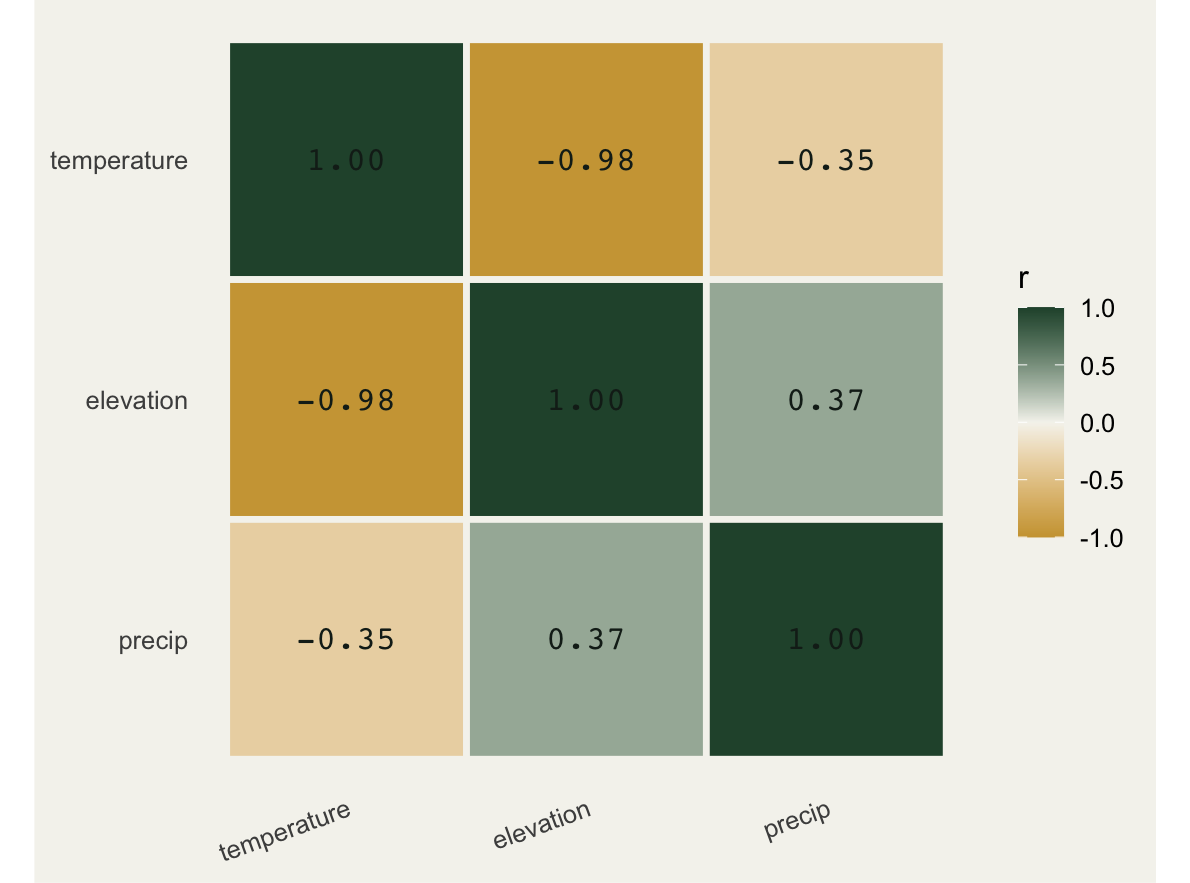
The full model hides the real effect
Fit the response on all three predictors and read the temperature coefficient.
m_full <- lm(carbon ~ temperature + elevation + precip, data = dat)
round(summary(m_full)$coefficients, 3)
Estimate Std. Error t value Pr(>|t|)
(Intercept) 19.173 10.767 1.781 0.079
temperature 0.286 0.447 0.639 0.525
elevation -0.004 0.003 -1.502 0.137
precip 0.002 0.002 1.024 0.309The true temperature effect is 0.9. The full model estimates it at 0.29 with a standard error of 0.45, a t value below one, and a p value of 0.52. On this evidence you would conclude temperature does not matter. It matters a great deal; the standard error is just too large to see it, because elevation is soaking up the same variation.
VIF from first principles
The variance inflation factor measures, for each predictor, how much of its variance is explained by the other predictors. Regress predictor j on all the others, take the resulting R squared, and:
\[\text{VIF}_j = \frac{1}{1 - R_j^2}\]
A predictor unrelated to the rest has R squared near zero and VIF near one. A predictor fully explained by the others has R squared near one and VIF heading to infinity. You do not need a package for this; it is a few lines of base R.
vif_manual <- function(model) {
  X <- model.matrix(model)[, -1, drop = FALSE]   # drop the intercept column
  preds <- colnames(X)
  out <- setNames(numeric(length(preds)), preds)
  for (p in preds) {
    others <- setdiff(preds, p)
    r2 <- summary(lm(X[, p] ~ X[, others, drop = FALSE]))$r.squared
    out[p] <- 1 / (1 - r2)
  }
  out
}
round(vif_manual(m_full), 2)
temperature elevation precip
23.27 23.64 1.16 Temperature and elevation both score around 23; precipitation sits at 1.2. The two collinear predictors are flagged loudly, the innocent one is not.
There is a clean interpretation of the number. The standard error of a coefficient is proportional to the square root of its VIF, so a VIF of 23 inflates the standard error by a factor of about 4.8 relative to the orthogonal case. That square root is the quantity to keep in mind: a VIF of 4 doubles the standard error, a VIF of 9 triples it. The damage to your error bars grows with the square root, not the raw VIF.
v <- vif_manual(m_full)
vd <- data.frame(pred = factor(names(v), levels = names(v)[order(v)]),
                 vif = as.numeric(v))
ggplot(vd, aes(vif, pred)) +
  geom_col(fill = "#275139", width = 0.6) +
  geom_vline(xintercept = 5, linetype = "dashed", colour = "#cda23f", linewidth = 0.7) +
  geom_vline(xintercept = 10, linetype = "dotted", colour = "#b5534e", linewidth = 0.8) +
  geom_text(aes(label = sprintf("%.1f", vif)), hjust = -0.2,
            colour = "#16241d", size = 4, family = "mono") +
  scale_x_continuous(expand = expansion(mult = c(0, 0.18))) +
  labs(x = "VIF", y = NULL) +
  theme_minimal(base_size = 12) +
  theme(panel.grid.minor = element_blank(),
        plot.background = element_rect(fill = "#f5f4ee", colour = NA),
        panel.background = element_rect(fill = "#f5f4ee", colour = NA))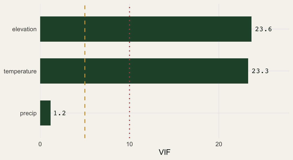
The fix: drop the redundant predictor
Elevation and temperature carry the same signal, so keep the one you can interpret and drop the other. Here temperature is the mechanistic driver, so elevation goes.
m_red <- lm(carbon ~ temperature + precip, data = dat)
round(summary(m_red)$coefficients, 3)
Estimate Std. Error t value Pr(>|t|)
(Intercept) 3.654 3.056 1.196 0.235
temperature 0.940 0.100 9.427 0.000
precip 0.002 0.002 0.820 0.415round(vif_manual(m_red), 2)temperature precip
1.14 1.14 Now temperature is estimated at 0.94, almost exactly the true 0.9, with a standard error of 0.10 and a p value below 0.001. The VIFs drop to 1.1. The effect was there the whole time; removing the redundant predictor let the model see it.
The standard error on temperature fell from 0.45 to 0.10, a factor of about 4.5, which is the square root of the VIF playing out in practice. The interval below makes the same point visually: the full model cannot rule out zero, while the reduced model lands tightly on the truth.
ci_f <- confint(m_full)["temperature", ]; est_f <- coef(m_full)["temperature"]
ci_r <- confint(m_red)["temperature", ];  est_r <- coef(m_red)["temperature"]
fd <- data.frame(
  model = factor(c("full (with elevation)", "reduced (no elevation)"),
                 levels = c("reduced (no elevation)", "full (with elevation)")),
  est = c(est_f, est_r), lo = c(ci_f[1], ci_r[1]), hi = c(ci_f[2], ci_r[2]))
ggplot(fd, aes(est, model)) +
  geom_vline(xintercept = 0.9, linetype = "dashed", colour = "#93a87f", linewidth = 0.7) +
  geom_vline(xintercept = 0, colour = "#dad9ca", linewidth = 0.5) +
  geom_errorbarh(aes(xmin = lo, xmax = hi), height = 0.16, colour = "#275139", linewidth = 0.9) +
  geom_point(size = 3.4, colour = "#275139") +
  annotate("text", x = 0.9, y = 2.42, label = "true value = 0.9",
           colour = "#46604a", size = 3.3, family = "mono", hjust = 0.5) +
  scale_x_continuous(expand = expansion(mult = c(0.05, 0.08))) +
  labs(x = "temperature coefficient (95% CI)", y = NULL) +
  theme_minimal(base_size = 12) +
  theme(panel.grid.minor = element_blank(),
        plot.background = element_rect(fill = "#f5f4ee", colour = NA),
        panel.background = element_rect(fill = "#f5f4ee", colour = NA))
Warning: `geom_errorbarh()` was deprecated in ggplot2 4.0.0.
ℹ Please use the `orientation` argument of `geom_errorbar()` instead.`height` was translated to `width`.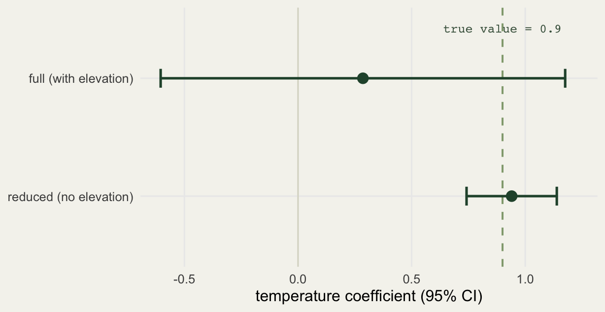
Prediction was never the problem
Here is the part that surprises people. The full model and the reduced model make almost identical predictions.
round(cor(predict(m_full), predict(m_red)), 3) # agreement of fitted values[1] 0.989round(max(abs(predict(m_full) - predict(m_red))), 2) # largest discrepancy[1] 1.58round(c(full = summary(m_full)$adj.r.squared,
reduced = summary(m_red)$adj.r.squared), 2) # adjusted R squared full reduced
0.55 0.54 The fitted values correlate at 0.99 and never differ by more than 1.6 units. The adjusted R squared is 0.55 for the full model and 0.54 for the reduced one. Collinearity scrambles the attribution of effect to individual predictors; it leaves the joint prediction essentially untouched. If your only goal is to predict the response, collinearity is mostly harmless. If you want to say which predictor matters and by how much, it is the whole ballgame.
Practical guidance
A few rules that hold up in ecological practice:
There is no universal VIF cutoff. A VIF above 5 is a common warning line and above 10 a common action line, but these are conventions, not laws. Graham 2003 showed that even modest predictor correlations (r at or above 0.28) can already distort multiple regression, so do not treat a VIF of 4 as automatically safe when interpretation matters.
When you find collinearity, you have three honest options: drop one predictor from each correlated cluster (keep the one you can interpret or measure reliably), combine the cluster into a composite axis (a principal component, see the PCA post), or accept that the cluster acts as a single block and stop trying to separate its members. What you should not do is keep all of them and read the individual coefficients as if collinearity were not there.
VIF is a property of the predictors, not of the response distribution. The same calculation applies to a Poisson or binomial GLM: compute it on the model’s design matrix exactly as above. Collinearity diagnostics transfer across the generalised linear model family unchanged.
Watch out for collinearity you create yourself. Interaction terms and polynomial terms are correlated with their components by construction; centring the predictors before forming products removes most of that artificial inflation. A high VIF on an interaction term is often an artefact of scaling rather than a real problem.
Finally, the most important habit: look at your predictors before you fit. A correlation matrix and a VIF take three lines of code and save you from confidently misreading a model that the data could never have answered. Zuur and colleagues make exactly this case in their data exploration protocol, and Dormann and colleagues review the fuller toolbox for when dropping variables is not enough.
References
Dormann et al. 2013 Ecography 36(1):27-46 (10.1111/j.1600-0587.2012.07348.x)
Graham 2003 Ecology 84(11):2809-2815 (10.1890/02-3114)
Zuur, Ieno and Elphick 2010 Methods in Ecology and Evolution 1(1):3-14 (10.1111/j.2041-210X.2009.00001.x)