Ridge regression for collinear predictors

Ridge regression stabilises least squares when ecological predictors are collinear and numerous: shrinkage, choosing the penalty, and the bias it buys.

Field studies rarely hand you a tidy set of independent predictors. You measure temperature, precipitation, a greenness index, soil moisture, a topographic wetness proxy and a dozen more, and most of them move together. Then you fit a linear model with more candidate layers than you have sites, and ordinary least squares (OLS) does something unhelpful: the coefficients swing to large, contradictory values and the standard errors blow up. Ridge regression is the standard first response. It adds a penalty on coefficient size, which trades a little bias for a large reduction in variance.

This post builds ridge from the closed form, chooses the penalty two ways, and is honest about what the shrinkage costs. It follows on from collinearity and VIF, which diagnosed the problem, and from penalised regression splines, which used exactly the same quadratic penalty in a smoothing context.

A predictor-heavy ecological design

We simulate 40 sites and 25 candidate environmental predictors driven by three latent gradients, so the predictors are intercorrelated the way real climate and terrain layers are. Ten predictors carry a small to moderate effect; the rest are noise layers a modeller might have thrown in.

library(ggplot2)

te_ink <- "#275139"; te_naive <- "#b5482a"; te_truth <- "#565656"
theme_te <- function(base_size = 12) {
  theme_minimal(base_size = base_size, base_family = "sans") +
    theme(plot.title = element_text(colour = te_ink, face = "bold"),
          plot.subtitle = element_text(colour = "#3f3f3f"),
          axis.title = element_text(colour = te_ink),
          panel.grid.minor = element_blank(),
          panel.grid.major = element_line(colour = "#e4dfd4", linewidth = 0.35),
          legend.position = "top")
}
theme_set(theme_te())

set.seed(4210)
n <- 40; p <- 25; ntest <- 8000
gen_X <- function(n) {
  f1 <- rnorm(n); f2 <- rnorm(n); f3 <- rnorm(n)
  M <- matrix(rnorm(n * p, 0, 1), n, p)
  M[, 1:9]   <- M[, 1:9]   * 0.55 + f1 * 0.85
  M[, 10:17] <- M[, 10:17] * 0.60 + f2 * 0.80
  M[, 18:25] <- M[, 18:25] * 0.70 + f3 * 0.70
  colnames(M) <- paste0("x", 1:p); M
}
X  <- gen_X(n)
beta_true <- c(0.55, 0.45, 0.40, 0, 0, 0.35, 0, 0, 0,
               0.60, 0.40, 0, 0, 0.35, 0, 0, 0,
               0.50, 0, 0, 0.30, 0, 0, 0, 0)
sigma <- 1.8
y  <- as.numeric(X %*% beta_true) + rnorm(n, 0, sigma)
Xt <- gen_X(ntest)
yt <- as.numeric(Xt %*% beta_true) + rnorm(ntest, 0, sigma)

The predictors are correlated but not degenerate, and there are more of them than the design comfortably supports.

cc <- cor(X)
mean_abs_cor <- mean(abs(cc[upper.tri(cc)]))

dfr <- data.frame(y = y, X)
ols <- lm(y ~ ., data = dfr)
b_ols <- coef(ols)[-1]

# variance inflation for x1 (the diagnostic from the collinearity post)
vif1 <- 1 / (1 - summary(lm(x1 ~ . - y, data = dfr))$r.squared)

# out-of-sample prediction error on the independent test set
rmse_ols <- sqrt(mean((yt - cbind(1, Xt) %*% coef(ols))^2))

With 40 sites and 25 predictors, OLS keeps only 14 residual degrees of freedom. The variance inflation factor for the first predictor is 9.1, so its standard error is roughly 3 times what it would be under independence. The largest fitted coefficient reaches 1.75 where the true effects never exceed 0.6.

The ridge estimator

Ridge minimises the residual sum of squares plus a penalty on the squared coefficients, lambda times the sum of the squared standardised slopes. The solution is a closed form, (X'X + lambda I)^-1 X' y, computed here through the singular value decomposition so the whole penalty path is one line. Two habits matter. Standardise the predictors first, otherwise the penalty depends on the arbitrary units of each layer; and leave the intercept out of the penalty by centring the response.

xm <- colMeans(X); xs <- apply(X, 2, sd); ym <- mean(y)
Xs <- scale(X, xm, xs)        # standardised predictors
yc <- y - ym                  # centred response
sv <- svd(Xs); d <- sv$d

# standardised ridge coefficients at penalty lambda
beta_std <- function(lambda) as.numeric(sv$v %*% ((d / (d^2 + lambda)) * (t(sv$u) %*% yc)))

# effective degrees of freedom = trace of the hat matrix
edf <- function(lambda) sum(d^2 / (d^2 + lambda))

# generalised cross-validation score
rss <- function(lambda) { b <- beta_std(lambda); sum((yc - Xs %*% b)^2) }
gcv <- function(lambda) { e <- edf(lambda); n * rss(lambda) / (n - e)^2 }

lam_grid <- exp(seq(log(1e-2), log(1e4), length.out = 500))
lam_gcv  <- lam_grid[which.min(sapply(lam_grid, gcv))]
edf_gcv  <- edf(lam_gcv)

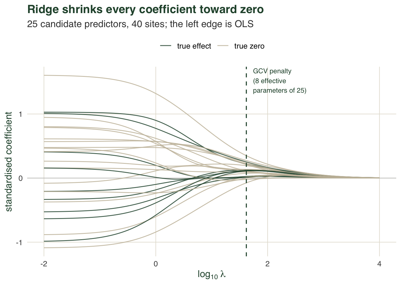
As the penalty grows, the effective degrees of freedom fall from the full 25 toward zero. Generalised cross-validation (GCV) picks lambda = 41.6, which corresponds to only 8 effective parameters. Every coefficient is pulled toward zero, and the tightly correlated predictors, which OLS could not separate, are shrunk together.

Figure 1: Ridge coefficient paths. Each of the 25 standardised coefficients (green: a true effect; tan: a true zero) shrinks toward zero as the penalty grows. The left edge is OLS, where the correlated predictors take large, contradictory values; the dashed line is the GCV penalty.

Choosing the penalty, and checking the choice

GCV is convenient because it needs one fit. A ten-fold cross-validation, standardising inside each training fold so no test information leaks, gives a nearly identical answer.

set.seed(77)
K <- 10; foldid <- sample(rep(1:K, length.out = n))
cv_rmse <- function(lambda) {
  err <- numeric(K)
  for (k in 1:K) {
    tr <- foldid != k; te <- !tr
    xmk <- colMeans(X[tr, ]); xsk <- apply(X[tr, ], 2, sd); ymk <- mean(y[tr])
    Xsk <- scale(X[tr, ], xmk, xsk); yck <- y[tr] - ymk; svk <- svd(Xsk)
    bk <- svk$v %*% ((svk$d / (svk$d^2 + lambda)) * (t(svk$u) %*% yck))
    bok <- bk / xsk; itk <- ymk - sum(bok * xmk)
    err[k] <- sum((y[te] - (as.numeric(X[te, , drop = FALSE] %*% bok) + itk))^2)
  }
  sqrt(sum(err) / n)
}
lam_cv <- lam_grid[which.min(sapply(lam_grid, cv_rmse))]

Cross-validation lands on lambda = 38.3, close to the GCV value of 41.6. The two selectors agreeing is reassuring, though neither is guaranteed to recover the penalty that minimises true error.

What the penalty buys

The point of ridge is prediction. On the independent test set, we compare OLS against ridge across the penalty path, back-transforming the standardised coefficients to the original scale.

test_rmse <- function(lambda) {
  b <- beta_std(lambda); bo <- b / xs; it <- ym - sum(bo * xm)
  sqrt(mean((yt - (as.numeric(Xt %*% bo) + it))^2))
}
trmse      <- sapply(lam_grid, test_rmse)
rmse_ridge <- test_rmse(lam_gcv)
lam_best   <- lam_grid[which.min(trmse)]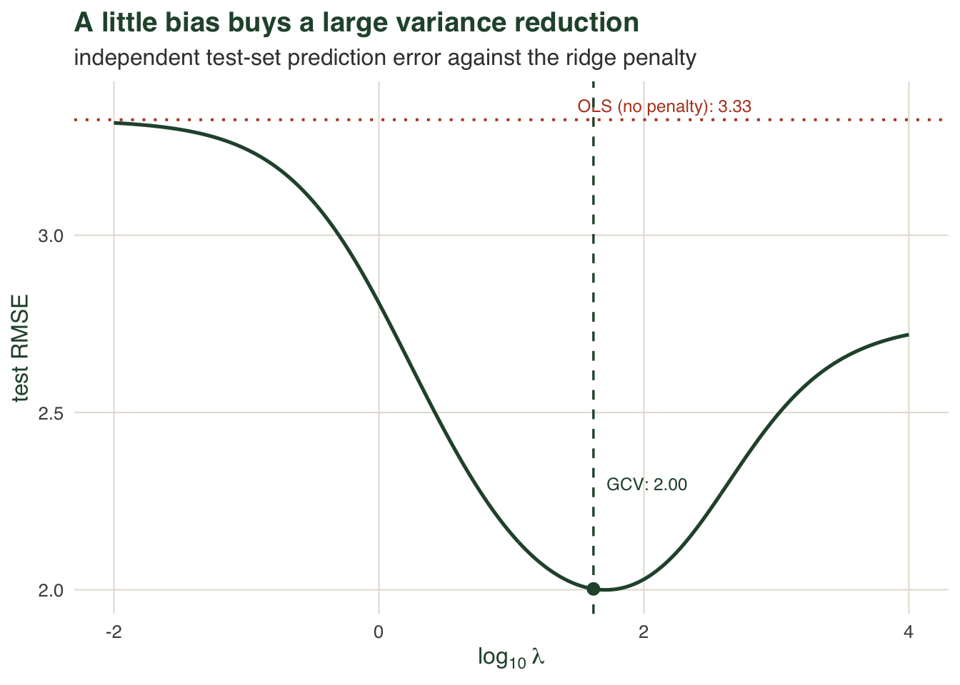

Figure 2: Bias-variance trade-off. Independent test error against the ridge penalty. OLS (the dotted line) overfits the 25 predictors; a moderate penalty cuts the error sharply, and the GCV choice sits near the minimum.

OLS predicts at RMSE 3.33; ridge at the GCV penalty predicts at 2, a factor of 1.66 better, and the GCV penalty is close to the test-optimal one (51.9). The stability of the coefficients tells the same story from the other side. Bootstrap the design and refit both estimators.

set.seed(101)
B <- 2000; bo1 <- br1 <- numeric(B)
for (b in 1:B) {
  idx <- sample.int(n, n, replace = TRUE); Xb <- X[idx, ]; yb <- y[idx]
  bo1[b] <- tryCatch(coef(lm(yb ~ Xb))[2], error = function(e) NA)
  xmb <- colMeans(Xb); xsb <- apply(Xb, 2, sd); ymb <- mean(yb)
  Xsb <- scale(Xb, xmb, xsb); ycb <- yb - ymb; svb <- svd(Xsb)
  br1[b] <- (svb$v %*% ((svb$d / (svb$d^2 + lam_gcv)) * (t(svb$u) %*% ycb)))[1]
}
flip      <- 100 * mean(bo1 < 0, na.rm = TRUE)
iqr_ols   <- IQR(bo1, na.rm = TRUE)
iqr_ridge <- IQR(br1)

The OLS coefficient on the first predictor swings from strongly negative to strongly positive, flipping sign in 33 percent of resamples for an effect that is truly positive; the ridge coefficient barely moves. Its interquartile range across resamples is 4.3 for OLS against 0.09 for ridge. The naive fit carries almost no usable information about that predictor; the penalised fit is stable.

The honest limits

Ridge is not a free upgrade, and three points deserve saying plainly.

First, the shrinkage is bias. Compare the length of the coefficient vector on the standardised scale.

norm_ols   <- sqrt(sum((b_ols * xs)^2))
norm_true  <- sqrt(sum((beta_true * xs)^2))
norm_ridge <- sqrt(sum(beta_std(lam_gcv)^2))

OLS produces a vector of length 3.53, inflated well past the truth (1.13) by collinearity. Ridge produces 0.79, shrunk below the truth. That is deliberate: pulling the estimates in reduces their variance more than it adds bias, which is why prediction improves. But it means a ridge coefficient is not an unbiased effect size. If your question is how large each driver is, ridge answers a different question than you asked.

Second, ridge does not select. Every one of the 25 coefficients stays nonzero, including the fifteen that are truly zero. Ridge stabilises a model; it does not tell you which predictors belong in it. That is what the L1 penalty does, in the next post on the lasso.

Third, the usual standard errors and p-values do not transfer. The penalty distorts the sampling distribution, and the coefficients are biased, so the ordinary regression table is not valid here. Quantifying uncertainty for a penalised fit needs its own care, which is the subject of checking a penalised regression.

Ridge earns its place when you have more correlated candidate predictors than your data can pin down and you want a stable model that predicts well. Read it as a prediction tool that buys variance reduction with honest bias, not as a cleaner route to effect sizes.

Related tutorials

• Lasso and variable selection
• Elastic net and cross-validation
• Collinearity and VIF
• Penalised regression splines

References

• Hoerl, A.E. and Kennard, R.W. 1970. Technometrics 12(1):55-67 (10.1080/00401706.1970.10488634)
• Reineking, B. and Schroder, B. 2006. Ecological Modelling 193(3-4):675-690 (10.1016/j.ecolmodel.2005.05.016)
• Dormann, C.F. et al. 2013. Ecography 36(1):27-46 (10.1111/j.1600-0587.2012.07348.x)
• Copas, J.B. 1983. Journal of the Royal Statistical Society B 45(3):311-354 (10.1111/j.2517-6161.1983.tb01258.x)
• Hastie, T., Tibshirani, R. and Friedman, J. 2009. The Elements of Statistical Learning, 2nd ed. Springer. ISBN 978-0-387-84857-0
• Harrell, F.E. 2015. Regression Modeling Strategies, 2nd ed. Springer. ISBN 978-3-319-19424-0