Lasso and variable selection

The lasso adds an L1 penalty that sets coefficients exactly to zero, doing selection and shrinkage at once. How it works, and why the selected set is unstable.

Ridge stabilises a collinear design but keeps every predictor in the model. Often the ecological question is the opposite one: out of thirty candidate layers, which few actually matter? The lasso answers that. It swaps ridge’s squared penalty for a penalty on the absolute size of the coefficients, and that single change lets it set coefficients to exactly zero. One fit both shrinks and selects.

This post builds the lasso by coordinate descent, chooses the penalty by cross-validation, and then makes an uncomfortable point honestly: the set of predictors the lasso keeps is not stable. It follows on from ridge regression, which introduced the penalty idea and the same predictor-heavy design, and it sets up elastic net and checking a penalised regression.

A predictor-heavy ecological design

We simulate 60 sites and 30 candidate predictors organised as three environmental gradients of ten layers each, so predictors within a gradient are correlated the way temperature, a greenness index and soil moisture would be. Six predictors carry a real effect; the other twenty-four are noise a modeller might have measured anyway.

library(ggplot2)

te_ink <- "#275139"; te_naive <- "#b5482a"; te_truth <- "#565656"
theme_te <- function(base_size = 12) {
  theme_minimal(base_size = base_size, base_family = "sans") +
    theme(plot.title = element_text(colour = te_ink, face = "bold"),
          plot.subtitle = element_text(colour = "#3f3f3f"),
          axis.title = element_text(colour = te_ink),
          panel.grid.minor = element_blank(),
          panel.grid.major = element_line(colour = "#e4dfd4", linewidth = 0.35),
          legend.position = "top")
}
theme_set(theme_te())

set.seed(4211)
n <- 60; p <- 30; ntest <- 8000; load <- 0.55; sigma <- 1.4
gen_X <- function(n) {
  f <- matrix(rnorm(n * 3), n, 3)
  M <- matrix(rnorm(n * p), n, p)
  for (g in 1:3) {
    idx <- ((g - 1) * 10 + 1):(g * 10)
    M[, idx] <- M[, idx] * sqrt(1 - load^2) + f[, g] * load
  }
  colnames(M) <- paste0("x", 1:p); M
}
X <- gen_X(n)
beta_true <- numeric(p)
beta_true[c(1, 5, 9, 17, 21, 25)] <- c(1.0, 0.75, 0.55, 0.8, 0.6, 0.7)
k_true <- sum(beta_true != 0)
y  <- as.numeric(X %*% beta_true) + rnorm(n, 0, sigma)
Xt <- gen_X(ntest)
yt <- as.numeric(Xt %*% beta_true) + rnorm(ntest, 0, sigma)

The lasso estimator

The lasso minimises the residual sum of squares plus lambda times the sum of the absolute standardised slopes. There is no closed form, but the L1 penalty has a tidy consequence: for one coefficient with the others held fixed, the update is soft-thresholding, taking the least-squares value and pulling it toward zero by lambda, and snapping it to exactly zero once it is inside that band. Cycling that update over the coefficients until nothing moves is coordinate descent, the same algorithm glmnet uses. As with ridge, standardise the predictors first so the penalty does not depend on each layer’s units, and centre the response so the intercept escapes the penalty.

soft <- function(z, g) sign(z) * pmax(abs(z) - g, 0)

lasso_fit <- function(Xs, yc, lambda, b0 = NULL, maxit = 10000, tol = 1e-9) {
  n <- nrow(Xs); p <- ncol(Xs); b <- if (is.null(b0)) numeric(p) else b0
  r <- yc - Xs %*% b
  for (it in 1:maxit) {
    dmax <- 0; bmax <- 0
    for (j in 1:p) {
      bj <- b[j]; rj <- r + Xs[, j] * bj
      bn <- soft(mean(Xs[, j] * rj), lambda); d <- bn - bj
      if (d != 0) { r <- rj - Xs[, j] * bn; b[j] <- bn }
      dmax <- max(dmax, abs(d)); bmax <- max(bmax, abs(bn))
    }
    if (dmax < tol * max(bmax, 1e-8)) break
  }
  b
}

lasso_path <- function(Xs, yc, lams) {
  P <- matrix(0, length(lams), ncol(Xs)); b <- NULL
  for (i in seq_along(lams)) { b <- lasso_fit(Xs, yc, lams[i], b0 = b); P[i, ] <- b }
  P
}

standardise <- function(X) {
  xm <- colMeans(X); Xc <- sweep(X, 2, xm)
  xn <- sqrt(colMeans(Xc^2))
  list(Xs = sweep(Xc, 2, xn, "/"), xm = xm, xn = xn)
}
back <- function(bs, xn, xm, ym) { bo <- bs / xn; list(bo = bo, it = ym - sum(bo * xm)) }

cc <- cor(X); mean_abs_cor <- mean(abs(cc[upper.tri(cc)]))
wg <- c()
for (g in 1:3) { idx <- ((g - 1) * 10 + 1):(g * 10); sub <- cc[idx, idx]; wg <- c(wg, sub[upper.tri(sub)]) }
wg_mean <- mean(abs(wg)); wg_max <- max(abs(wg))

st <- standardise(X); ym <- mean(y); yc <- y - ym
lam_max  <- max(abs(colMeans(st$Xs * yc)))         # smallest penalty killing every coefficient
lam_grid <- exp(seq(log(lam_max), log(lam_max * 1e-3), length.out = 100))
P <- lasso_path(st$Xs, yc, lam_grid)

ols <- lm(y ~ ., data = data.frame(y = y, X))
rmse_ols <- sqrt(mean((yt - cbind(1, Xt) %*% coef(ols))^2))

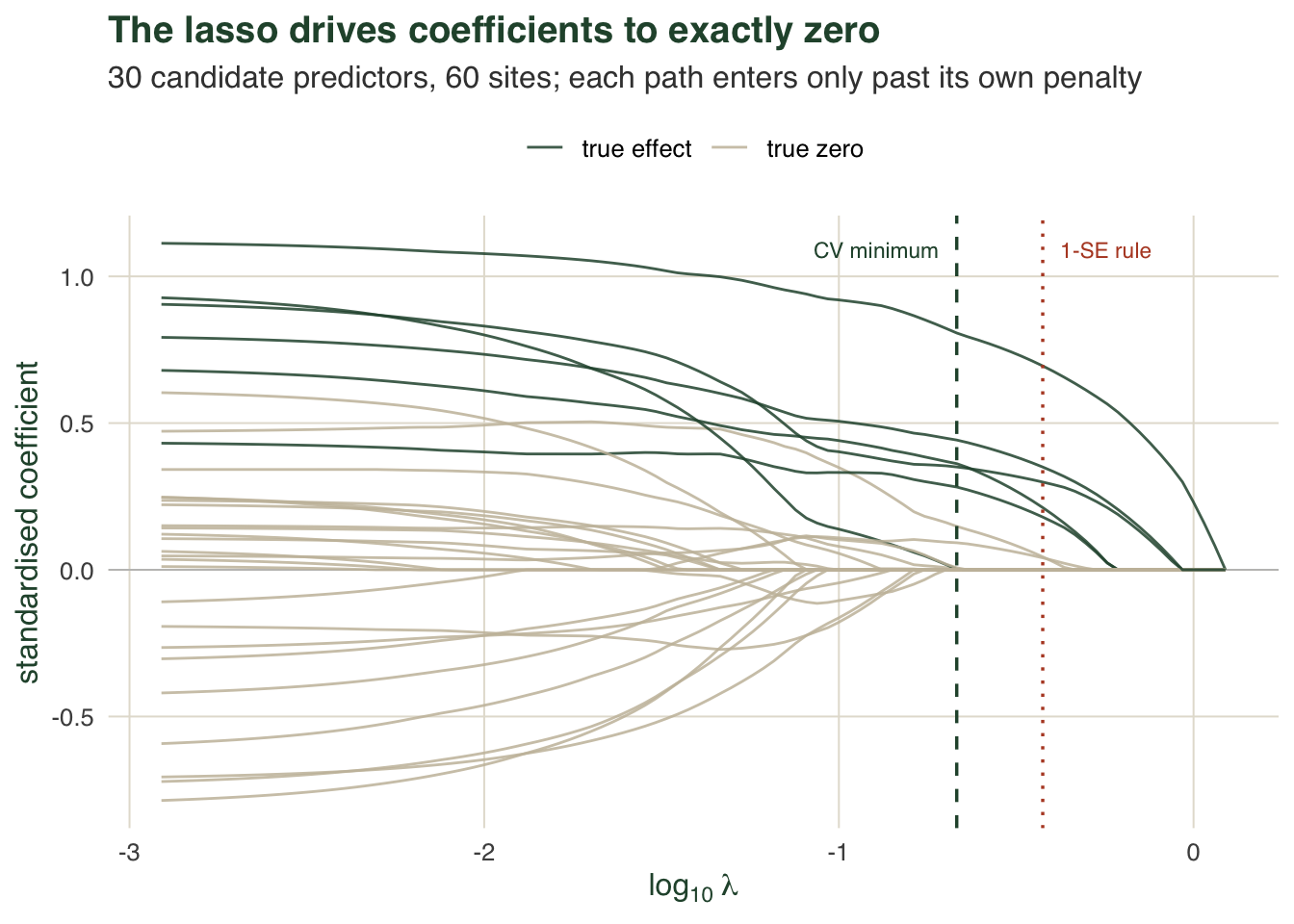
Predictors within a gradient correlate about 0.28 on average and up to 0.55, while across the whole matrix the mean absolute correlation is 0.15. With 60 sites and 30 predictors, ordinary least squares keeps only 29 residual degrees of freedom and overfits badly. The penalty path runs from lambda = 1.23, where every coefficient is zero, down toward the least-squares fit on the left.

Choosing the penalty

The penalty is chosen by prediction error, not by looking at the coefficients. Ten-fold cross-validation, standardising inside each training fold so no test information leaks, gives two conventional choices: the penalty at the minimum cross-validated error, and the largest penalty within one standard error of that minimum, which deliberately selects a smaller model.

cv_lasso <- function(X, y, lams, K = 10, seed = 1) {
  set.seed(seed); n <- nrow(X)
  fold <- sample(rep(1:K, length.out = n)); E <- matrix(NA, K, length(lams))
  for (kk in 1:K) {
    tr <- fold != kk; te <- !tr
    s <- standardise(X[tr, ]); yct <- y[tr] - mean(y[tr])
    Ptr <- lasso_path(s$Xs, yct, lams)
    for (i in seq_along(lams)) {
      q <- back(Ptr[i, ], s$xn, s$xm, mean(y[tr]))
      E[kk, i] <- mean((y[te] - (as.numeric(X[te, , drop = FALSE] %*% q$bo) + q$it))^2)
    }
  }
  cvm <- colMeans(E); cvse <- apply(E, 2, sd) / sqrt(K)
  im <- which.min(cvm); i1 <- min(which(cvm <= cvm[im] + cvse[im]))
  list(im = im, i1 = i1, lm = lams[im], l1 = lams[i1])
}
cv <- cv_lasso(X, y, lam_grid, K = 10, seed = 4311)
b_min <- P[cv$im, ]; b_1se <- P[cv$i1, ]
sel_min <- which(b_min != 0); sel_1se <- which(b_1se != 0)
tp <- function(s) sum(beta_true[s] != 0); fp <- function(s) sum(beta_true[s] == 0)

The minimum sits at lambda = 0.215 and keeps 10 predictors: 6 of the six real effects and 4 false ones. The one-standard-error penalty, lambda = 0.376, trims to 7 predictors, 5 true and 2 false. Both figures below mark these two choices on the coefficient paths.

Figure 1: Lasso coefficient paths. Each of the 30 standardised coefficients (green: a true effect; tan: a true zero) stays flat at zero until the penalty drops past its entry point. The dashed line is the cross-validation minimum; the dotted line is the one-standard-error rule.

What the selection buys, and against what

Ridge would keep all thirty predictors here. To see what selection is worth, compare four fits on an independent test set: least squares, a ridge fit chosen by generalised cross-validation, and the lasso at each of the two penalties.

sv <- svd(st$Xs); d <- sv$d
ridge_std <- function(l) as.numeric(sv$v %*% ((d / (d^2 + l)) * (t(sv$u) %*% yc)))
edf_r <- function(l) sum(d^2 / (d^2 + l))
gcv_r <- function(l) { e <- edf_r(l); n * sum((yc - st$Xs %*% ridge_std(l))^2) / (n - e)^2 }
lamr  <- exp(seq(log(1e-2), log(1e4), length.out = 400))
lam_r <- lamr[which.min(sapply(lamr, gcv_r))]
b_ridge <- ridge_std(lam_r); nz_ridge <- sum(b_ridge != 0)

trmse <- function(bs) { q <- back(bs, st$xn, st$xm, ym); sqrt(mean((yt - (as.numeric(Xt %*% q$bo) + q$it))^2)) }
rmse_ridge <- trmse(b_ridge); rmse_min <- trmse(b_min); rmse_1se <- trmse(b_1se)

Ridge keeps all 30 predictors and predicts at RMSE 1.77; least squares, overfit, sits at 2.32. The lasso at the CV minimum matches ridge on prediction, 1.75, using a handful of predictors instead of all thirty, and the sparser one-standard-error fit costs a little accuracy at 1.9. So the lasso buys a readable, sparse model at no real cost in prediction here. The catch is what that selected set means.

The selected set is unstable

The coefficient paths make selection look definite: a predictor is either in or out at a given penalty. Resampling the data tells a different story. We bootstrap the sites, refit the lasso at the CV-minimum penalty on each resample, and record how often each predictor is selected.

set.seed(4321); B <- 2000; sf <- numeric(p)
for (b in 1:B) {
  id <- sample.int(n, n, replace = TRUE)
  s <- standardise(X[id, ]); ycb <- y[id] - mean(y[id])
  sf <- sf + (lasso_fit(s$Xs, ycb, cv$lm) != 0)
}
sf <- sf / B
stable_tp <- sum(sf[beta_true != 0] > 0.9)
flick <- sum(sf > 0.2 & sf < 0.8)
x21_freq <- sf[21]                                     # a true effect of 0.6
maxnoise_var  <- which(beta_true == 0)[which.max(sf[beta_true == 0])]
maxnoise_name <- paste0("x", maxnoise_var)
maxnoise_freq <- max(sf[beta_true == 0])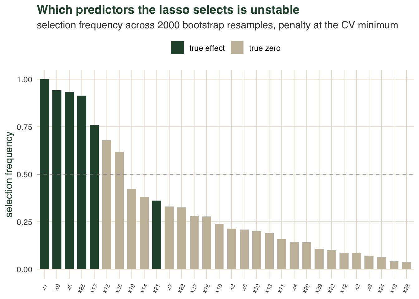

Figure 2: Selection frequency across 2000 bootstrap resamples at the CV-minimum penalty (green: a true effect; tan: a true zero). Only the strongest true effects are selected almost every time; weaker true effects and several noise predictors sit near the coin-flip line.

Only 4 of the six true effects are selected in more than ninety percent of resamples. A genuine effect of 0.6 on predictor 21 is selected in just 36 percent of them, less than a coin flip, because a correlated neighbour keeps standing in for it. Meanwhile x15, which is truly zero, is selected 68 percent of the time. Across all thirty predictors, 14 of them flicker between selected and dropped depending on the resample. The single selected set you get from one fit is one draw from this distribution, not a fact about the system.

The honest limits

The lasso is a strong tool for the question it answers, but three points deserve saying plainly.

First, the coefficients are still shrunk. Soft-thresholding pulls every surviving coefficient toward zero by the penalty, so a lasso estimate is biased toward zero and is not an unbiased effect size, exactly as with ridge. If you refit least squares on the selected predictors to remove that bias, you have used the data twice, and the second point below applies with full force.

Second, selection is unstable, and that instability is not noise to be averaged away. When predictors are correlated, the lasso tends to pick one from a group almost at random and drop the others, so a slightly different sample gives a different set. Reporting one selected model as the set of drivers overstates how much the data pin down. The grouping behaviour, and a partial remedy for it, is the subject of the elastic net; measuring selection stability directly through resampling belongs to checking a penalised regression.

Third, the usual standard errors and p-values do not transfer, and here the reason is sharper than for ridge. The predictors in your final table were chosen because they looked useful in this sample, so testing them with the ordinary formulae, as if the model had been fixed in advance, understates the uncertainty and overstates the significance. Valid inference after selection needs methods built for it, which is again the checking post.

The lasso earns its place when you have many candidate predictors and want a sparse, predictive model you can read. Trust it for prediction and for a shortlist of plausible drivers; do not read the selected set as the drivers, or the coefficients as their effect sizes.

Related tutorials

• Ridge regression for collinear predictors
• Elastic net and cross-validation
• Checking a penalised regression
• Collinearity and VIF

References

• Tibshirani, R. 1996. Journal of the Royal Statistical Society B 58(1):267-288 (10.1111/j.2517-6161.1996.tb02080.x)
• Zou, H. and Hastie, T. 2005. Journal of the Royal Statistical Society B 67(2):301-320 (10.1111/j.1467-9868.2005.00503.x)
• Friedman, J., Hastie, T. and Tibshirani, R. 2010. Journal of Statistical Software 33(1):1-22 (10.18637/jss.v033.i01)
• Meinshausen, N. and Buhlmann, P. 2010. Journal of the Royal Statistical Society B 72(4):417-473 (10.1111/j.1467-9868.2010.00740.x)
• Dormann, C.F. et al. 2013. Ecography 36(1):27-46 (10.1111/j.1600-0587.2012.07348.x)
• Hastie, T., Tibshirani, R. and Friedman, J. 2009. The Elements of Statistical Learning, 2nd ed. Springer. ISBN 978-0-387-84857-0
• Harrell, F.E. 2015. Regression Modeling Strategies, 2nd ed. Springer. ISBN 978-3-319-19424-0