Elastic net and cross-validation

The elastic net mixes the ridge and lasso penalties, keeping correlated predictors together where the lasso splits them, and is tuned by cross-validation over two knobs.

The lasso has a known weakness with the correlated predictors that fill ecological datasets: faced with a group of layers measuring nearly the same gradient, it tends to keep one and drop the rest, and which one it keeps changes from sample to sample. The elastic net was designed for exactly this. It penalises coefficients with a weighted blend of the lasso’s absolute penalty and ridge’s squared penalty, and the ridge part encourages correlated predictors to enter or leave together.

This post builds the elastic net by coordinate descent, tunes it by cross-validation over both the mixing weight and the penalty, and shows the grouping behaviour directly by resampling. It follows on from ridge and the lasso, and leads into checking a penalised regression.

A design with a correlated group

We simulate 60 sites and 30 predictors. Six of them form a tight group driven by one latent gradient and each carries the same real effect, the situation where the lasso struggles. Three further isolated predictors carry stronger effects, and the rest are noise.

library(ggplot2)

te_ink <- "#275139"; te_naive <- "#b5482a"; te_truth <- "#565656"
theme_te <- function(base_size = 12) {
  theme_minimal(base_size = base_size, base_family = "sans") +
    theme(plot.title = element_text(colour = te_ink, face = "bold"),
          plot.subtitle = element_text(colour = "#3f3f3f"),
          axis.title = element_text(colour = te_ink),
          panel.grid.minor = element_blank(),
          panel.grid.major = element_line(colour = "#e4dfd4", linewidth = 0.35),
          legend.position = "top")
}
theme_set(theme_te())

set.seed(4212)
n <- 60; p <- 30; ntest <- 8000; sigma <- 1.4
gen_X <- function(n) {
  f <- matrix(rnorm(n * 4), n, 4); M <- matrix(rnorm(n * p), n, p)
  M[, 1:6]   <- M[, 1:6]   * sqrt(1 - 0.9^2) + f[, 1] * 0.9   # the correlated group
  M[, 7:16]  <- M[, 7:16]  * sqrt(1 - 0.5^2) + f[, 2] * 0.5
  M[, 17:26] <- M[, 17:26] * sqrt(1 - 0.5^2) + f[, 3] * 0.5
  M[, 27:30] <- M[, 27:30] * sqrt(1 - 0.4^2) + f[, 4] * 0.4
  colnames(M) <- paste0("x", 1:p); M
}
X <- gen_X(n)
grp <- 1:6
beta_true <- numeric(p)
beta_true[grp] <- 0.45                          # six correlated members share the signal
beta_true[c(10, 20, 28)] <- c(0.8, 0.7, 0.6)    # isolated singletons
k_true <- sum(beta_true != 0)
y  <- as.numeric(X %*% beta_true) + rnorm(n, 0, sigma)
Xt <- gen_X(ntest); yt <- as.numeric(Xt %*% beta_true) + rnorm(ntest, 0, sigma)

The elastic net estimator

The elastic net minimises the residual sum of squares plus a penalty that mixes the two shapes: lambda sets the overall strength, and alpha between 0 and 1 sets the mix, so alpha = 1 is the lasso and alpha = 0 is ridge. On standardised predictors each coefficient has a tidy coordinate update, soft-threshold the least-squares value by lambda*alpha and then divide by 1 + lambda*(1-alpha); the numerator is the lasso’s selection, the denominator is ridge’s shrinkage. We compute this by coordinate descent with covariance updates, cycling until nothing moves, which is how glmnet does it.

soft <- function(z, g) sign(z) * pmax(abs(z) - g, 0)
en_fit_cov <- function(G, xy, lambda, alpha, b0 = NULL, maxit = 5000, tol = 1e-7) {
  p <- length(xy); b <- if (is.null(b0)) numeric(p) else b0
  denom <- 1 + lambda * (1 - alpha); g <- lambda * alpha
  cvec <- xy - as.numeric(G %*% b)           # c_j = X'y/n - (Gb)_j, kept in step with b
  for (it in 1:maxit) {
    dmax <- 0
    for (j in 1:p) {
      zj <- cvec[j] + b[j]
      bn <- soft(zj, g) / denom; d <- bn - b[j]
      if (d != 0) { cvec <- cvec - G[, j] * d; b[j] <- bn }
      dmax <- max(dmax, abs(d))
    }
    if (dmax < tol) break
  }
  b
}
gram_of <- function(Xs) crossprod(Xs) / nrow(Xs)
xy_of   <- function(Xs, yc) as.numeric(crossprod(Xs, yc)) / nrow(Xs)
en_path_cov <- function(G, xy, lams, alpha) {
  P <- matrix(0, length(lams), ncol(G)); b <- NULL
  for (i in seq_along(lams)) { b <- en_fit_cov(G, xy, lams[i], alpha, b0 = b); P[i, ] <- b }
  P
}
standardise <- function(X) {
  xm <- colMeans(X); Xc <- sweep(X, 2, xm); xn <- sqrt(colMeans(Xc^2))
  list(Xs = sweep(Xc, 2, xn, "/"), xm = xm, xn = xn)
}
back <- function(bs, xn, xm, ym) { bo <- bs / xn; list(bo = bo, it = ym - sum(bo * xm)) }
lam_max_a <- function(Xs, yc, alpha) max(abs(colMeans(Xs * yc))) / max(alpha, 0.05)

cc <- cor(X); gcor <- cc[grp, grp]; group_cor <- mean(gcor[upper.tri(gcor)])
st <- standardise(X); ym <- mean(y); yc <- y - ym
G0 <- gram_of(st$Xs); xy0 <- xy_of(st$Xs, yc)

The six group members correlate about 0.82 with one another, the kind of redundancy a set of climate layers would show. There are 9 true effects in all.

Tuning over the mix and the penalty

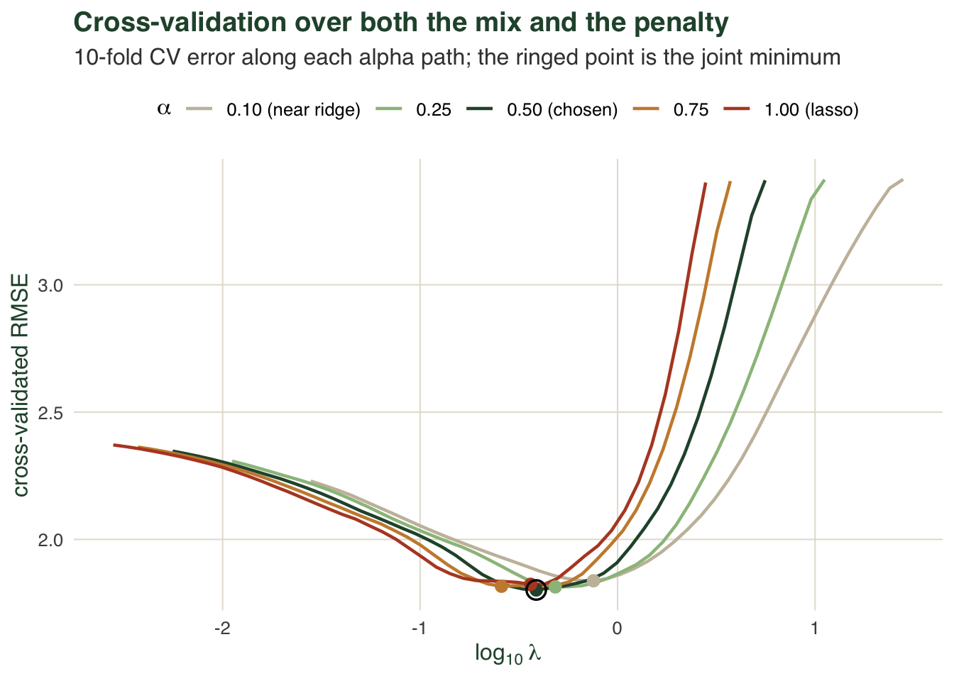
Both knobs are chosen by prediction error. For each alpha on a grid we run a ten-fold cross-validation over its own penalty path, using the same folds throughout so the comparison is fair, and take the pair that minimises cross-validated error.

alphas <- c(0.1, 0.25, 0.5, 0.75, 1.0)
nl <- 45
set.seed(4312); K <- 10; fold <- sample(rep(1:K, length.out = n))
folds <- lapply(1:K, function(kk) {
  tr <- fold != kk; s <- standardise(X[tr, ]); yct <- y[tr] - mean(y[tr])
  list(tr = tr, s = s, G = gram_of(s$Xs), xy = xy_of(s$Xs, yct), ytr = mean(y[tr]))
})
cv_alpha <- function(alpha) {
  lmax <- lam_max_a(st$Xs, yc, alpha)
  lams <- exp(seq(log(lmax), log(lmax * 1e-3), length.out = nl))
  E <- matrix(NA, K, nl)
  for (kk in 1:K) {
    fk <- folds[[kk]]; te <- !fk$tr
    Ptr <- en_path_cov(fk$G, fk$xy, lams, alpha)
    for (i in 1:nl) {
      q <- back(Ptr[i, ], fk$s$xn, fk$s$xm, fk$ytr)
      E[kk, i] <- mean((y[te] - (as.numeric(X[te, , drop = FALSE] %*% q$bo) + q$it))^2)
    }
  }
  cvm <- colMeans(E)
  data.frame(alpha = alpha, lam = lams, rmse = sqrt(cvm), cvm = cvm)
}
cvgrid <- do.call(rbind, lapply(alphas, cv_alpha))
best <- cvgrid[which.min(cvgrid$cvm), ]
amins <- do.call(rbind, lapply(split(cvgrid, cvgrid$alpha), function(d) d[which.min(d$cvm), ]))
amins <- amins[order(amins$alpha), ]
alpha_hat <- best$alpha; lam_hat <- best$lam
lam_las   <- amins$lam[amins$alpha == 1.0]
cv_spread <- max(amins$rmse) - min(amins$rmse)

Cross-validation prefers alpha = 0.5 at lambda = 0.387. That preference is mild, though: the best score at each alpha runs from 1.84 at the near-ridge end to 1.82 for the lasso, a span of only 0.036 in RMSE. The mixing weight is weakly identified, a point worth remembering before reporting it as though the data pinned it down.

Figure 1: Cross-validated error along each alpha path. The five curves are close, and the ringed point marks the joint minimum at alpha = 0.5. The flatness across alpha is the honest signal: the data prefer a blend, but only slightly over the lasso.

What the blend buys

Fit the chosen elastic net and the lasso, and compare both against ordinary least squares on the independent test set.

b_en  <- en_fit_cov(G0, xy0, lam_hat, alpha_hat)
b_las <- en_fit_cov(G0, xy0, lam_las, 1.0)
sel_en <- which(b_en != 0); sel_las <- which(b_las != 0)
grp_en <- sum(b_en[grp] != 0); grp_las <- sum(b_las[grp] != 0)
tp <- function(s) sum(beta_true[s] != 0); fp <- function(s) sum(beta_true[s] == 0)

trmse <- function(bs) { q <- back(bs, st$xn, st$xm, ym); sqrt(mean((yt - (as.numeric(Xt %*% q$bo) + q$it))^2)) }
ols <- lm(y ~ ., data = data.frame(y = y, X)); rmse_ols <- sqrt(mean((yt - cbind(1, Xt) %*% coef(ols))^2))
rmse_en <- trmse(b_en); rmse_las <- trmse(b_las)

On prediction the elastic net comes out ahead: test RMSE 1.66, against 1.81 for the lasso and 2.13 for the overfit least-squares model. The two selected sets differ in a telling way. The lasso keeps 7 predictors (7 true, 0 false) and picks up 5 of the six group members; the elastic net keeps 13 (9 true, 4 false) and keeps all 6 of the group. The blend recovers the whole correlated group, at the cost of admitting a few more false predictors.

The grouping effect, seen by resampling

One fit cannot show stability. We bootstrap the sites and refit both estimators at their chosen penalties, recording how often each of the six group members is selected.

set.seed(4322); B <- 800
sf_en <- numeric(p); sf_las <- numeric(p)
for (b in 1:B) {
  id <- sample.int(n, n, replace = TRUE)
  s <- standardise(X[id, ]); ycb <- y[id] - mean(y[id])
  G <- gram_of(s$Xs); xy <- xy_of(s$Xs, ycb)
  sf_en  <- sf_en  + (en_fit_cov(G, xy, lam_hat, alpha_hat) != 0)
  sf_las <- sf_las + (en_fit_cov(G, xy, lam_las, 1.0) != 0)
}
sf_en <- sf_en / B; sf_las <- sf_las / B
grp_freq_en  <- mean(sf_en[grp]);  grp_min_en  <- min(sf_en[grp])
grp_freq_las <- mean(sf_las[grp]); grp_min_las <- min(sf_las[grp])
worst_las <- paste0("x", grp[which.min(sf_las[grp])])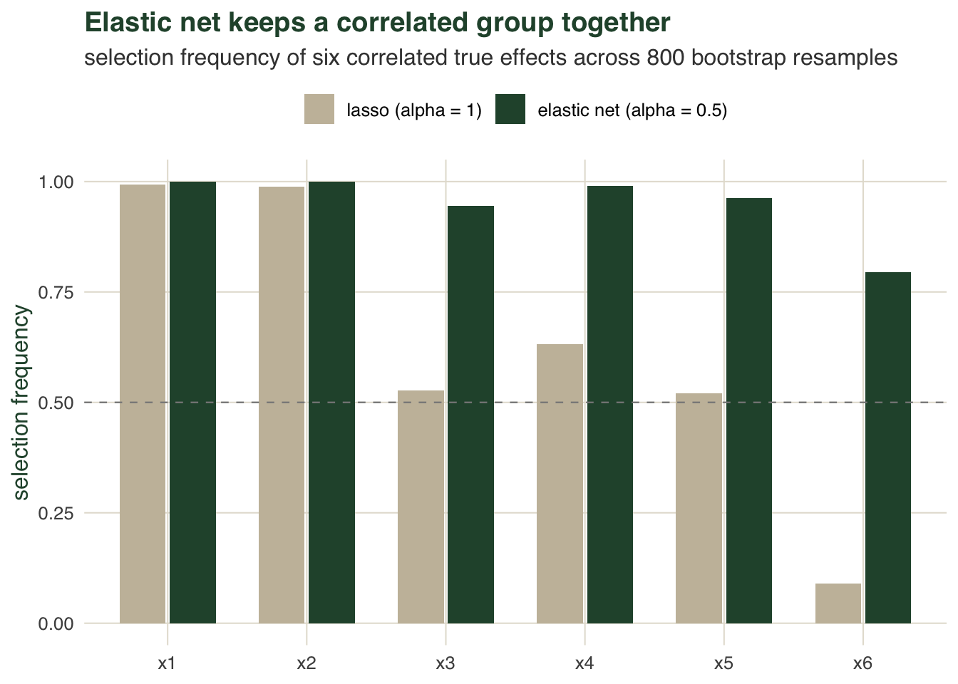

Figure 2: Selection frequency of the six correlated true effects across 800 bootstrap resamples. The elastic net selects them together in nearly every resample; the lasso keeps one or two and drops the others, the choice shifting between resamples.

The contrast is stark. The elastic net selects the group members in 95 percent of resamples on average, and even the weakest is kept 80 percent of the time. The lasso averages 62 percent across the same six, and drops one of them (x6) in all but 9 percent of resamples, standing a correlated neighbour in its place. Where the lasso reports an arbitrary one or two of the group, the elastic net reports the group.

The honest limits

The elastic net fixes one specific problem well, and it is worth being clear about what it does not fix.

First, the mixing weight is barely identified. The cross-validation surface here is nearly flat across alpha, so a slightly different sample, or different folds, could name a different alpha. Read the chosen mix as a mild preference for a blend, not as an estimated quantity, and if you report a single tuned model, remember that a plain ten-fold score understates the true error, because the tuning used the same data. An outer cross-validation loop around the whole selection is the honest way to quote predictive error.

Second, the stability the grouping buys costs sparsity. The elastic net keeps more predictors than the lasso, including more false ones, because the ridge part pulls correlated predictors in as a block whether or not they matter. That is the right trade when you care about not missing members of a real group, and the wrong one when you want the shortest honest list. It is a choice on the sparsity-stability axis, not a free improvement.

Third, the coefficients are still shrunk, and selection is still conditional on the data. The elastic net stabilises which predictors appear together; it does not make their coefficients unbiased effect sizes, and it does not license the ordinary standard errors and p-values, for the same reasons as ridge and the lasso. Quantifying uncertainty for the fitted model, and measuring how stable the selection really is, is the subject of checking a penalised regression.

The elastic net earns its place when your predictors come in correlated groups and you would rather keep a group whole than pick one member at random. Reach for it over the lasso when grouping matters; keep reading it as a prediction and screening tool, not as a route to effect sizes.

Related tutorials

• Ridge regression for collinear predictors
• Lasso and variable selection
• Checking a penalised regression
• Collinearity and VIF

References

• Zou, H. and Hastie, T. 2005. Journal of the Royal Statistical Society B 67(2):301-320 (10.1111/j.1467-9868.2005.00503.x)
• Tibshirani, R. 1996. Journal of the Royal Statistical Society B 58(1):267-288 (10.1111/j.2517-6161.1996.tb02080.x)
• Friedman, J., Hastie, T. and Tibshirani, R. 2010. Journal of Statistical Software 33(1):1-22 (10.18637/jss.v033.i01)
• Meinshausen, N. and Buhlmann, P. 2010. Journal of the Royal Statistical Society B 72(4):417-473 (10.1111/j.1467-9868.2010.00740.x)
• Dormann, C.F. et al. 2013. Ecography 36(1):27-46 (10.1111/j.1600-0587.2012.07348.x)
• Hastie, T., Tibshirani, R. and Friedman, J. 2009. The Elements of Statistical Learning, 2nd ed. Springer. ISBN 978-0-387-84857-0