Checking a penalised regression

The coefficient table from a lasso or elastic net does not support the usual confidence intervals. A coverage experiment shows why, and what to do instead.

The three previous posts fitted penalised models and each ended on the same warning: the coefficients are shrunk, the selected set is unstable, and the ordinary standard errors do not transfer. This post makes that warning concrete. We run a coverage experiment, the honest test of any confidence interval, and watch the naive intervals fail. Then we show a fix that works.

It closes the regularisation sequence from ridge, the lasso and the elastic net, and it uses the same coverage logic as the earlier honest-limits posts on checking a model after selection.

What a confidence interval promises

A 95% interval makes one promise: across repeated samples, it contains the true value 95% of the time. That is testable by simulation. We build a design where we know the truth, draw data many times, form intervals each time, and count how often they cover. Anything far below 95% is a broken interval.

library(ggplot2)

te_ink <- "#275139"; te_naive <- "#b5482a"; te_truth <- "#565656"
theme_te <- function(base_size = 12) {
  theme_minimal(base_size = base_size, base_family = "sans") +
    theme(plot.title = element_text(colour = te_ink, face = "bold"),
          plot.subtitle = element_text(colour = "#3f3f3f"),
          axis.title = element_text(colour = te_ink),
          panel.grid.minor = element_blank(),
          panel.grid.major = element_line(colour = "#e4dfd4", linewidth = 0.35),
          legend.position = "top")
}
theme_set(theme_te())

set.seed(4213)
n <- 100; p <- 30; sigma <- 2.0
nblk <- 6; blk <- 5
gen_X <- function(n) {
  M <- matrix(rnorm(n * p), n, p)
  for (bb in 1:nblk) { idx <- ((bb - 1) * blk + 1):(bb * blk)
    f <- rnorm(n); M[, idx] <- M[, idx] * sqrt(1 - 0.6^2) + f * 0.6 }   # correlated blocks
  colnames(M) <- paste0("x", 1:p); M
}
X <- gen_X(n)
beta_true <- numeric(p)
beta_true[c(1, 6, 16)] <- c(1.2, 1.0, 0.9)   # strong effects, one per block
beta_true[11] <- 0.5                          # the focal effect: moderate, near the selection boundary
focal <- 11
k_true <- sum(beta_true != 0)
mu <- as.numeric(X %*% beta_true)
cc <- cor(X); b3 <- cc[11:15, 11:15]; blk_cor <- mean(b3[upper.tri(b3)])

The predictors sit in six correlated blocks (within-block correlation about 0.39), and there are 4 true effects. The focal predictor, x11, carries a moderate effect of 0.5: strong enough to matter, weak enough that the lasso does not always select it. That is exactly the regime where inference goes wrong.

Fixing the penalty, and three ways to build an interval

We select with the lasso by coordinate descent, using the one-standard-error penalty from a pilot cross-validation, a common default. Holding the penalty fixed keeps the experiment about inference, not about tuning.

soft <- function(z, g) sign(z) * pmax(abs(z) - g, 0)
gram_of <- function(Xs) crossprod(Xs) / nrow(Xs)
xy_of   <- function(Xs, yc) as.numeric(crossprod(Xs, yc)) / nrow(Xs)
lasso_cov <- function(G, xy, lambda, b0 = NULL, maxit = 5000, tol = 1e-7) {
  p <- length(xy); b <- if (is.null(b0)) numeric(p) else b0
  cvec <- xy - as.numeric(G %*% b)
  for (it in 1:maxit) { dmax <- 0
    for (j in 1:p) { zj <- cvec[j] + b[j]; bn <- soft(zj, lambda); d <- bn - b[j]
      if (d != 0) { cvec <- cvec - G[, j] * d; b[j] <- bn }; dmax <- max(dmax, abs(d)) }
    if (dmax < tol) break }
  b
}
standardise <- function(X) { xm <- colMeans(X); Xc <- sweep(X, 2, xm)
  xn <- sqrt(colMeans(Xc^2)); list(Xs = sweep(Xc, 2, xn, "/"), xm = xm, xn = xn) }
lasso_coef_orig <- function(X, yv, lambda) {
  s <- standardise(X); yc <- yv - mean(yv)
  as.numeric(lasso_cov(gram_of(s$Xs), xy_of(s$Xs, yc), lambda)) / s$xn
}
## fast OLS: coefficients and classical standard errors on a chosen design
ols_cse <- function(Z, yv) {
  ch <- chol(crossprod(Z)); bhat <- backsolve(ch, forwardsolve(t(ch), crossprod(Z, yv)))
  r <- yv - Z %*% bhat; s2 <- sum(r^2) / (nrow(Z) - ncol(Z))
  list(b = as.numeric(bhat), se = sqrt(s2 * diag(chol2inv(ch))))
}

## pilot cross-validation to fix the one-standard-error penalty
set.seed(999); ypilot <- mu + rnorm(n, 0, sigma)
sp <- standardise(X); ycp <- ypilot - mean(ypilot)
lam_max <- max(abs(xy_of(sp$Xs, ycp)))
lam_grid <- exp(seq(log(lam_max), log(lam_max * 1e-3), length.out = 50))
K <- 10; set.seed(1001); fold <- sample(rep(1:K, length.out = n))
cvfold <- function(l, agg) {
  e <- numeric(K)
  for (kk in 1:K) { tr <- fold != kk; te <- !tr
    s <- standardise(X[tr, ]); yct <- ypilot[tr] - mean(ypilot[tr])
    bo <- as.numeric(lasso_cov(gram_of(s$Xs), xy_of(s$Xs, yct), l)) / s$xn
    it <- mean(ypilot[tr]) - sum(bo * s$xm)
    e[kk] <- mean((ypilot[te] - (as.numeric(X[te, , drop = FALSE] %*% bo) + it))^2) }
  agg(e)
}
cvm  <- sapply(lam_grid, cvfold, agg = mean)
cvse <- sapply(lam_grid, cvfold, agg = function(e) sd(e) / sqrt(K))
im <- which.min(cvm); i1 <- min(which(cvm <= cvm[im] + cvse[im]))
lam_1se <- lam_grid[i1]; frac_1se <- lam_1se / lam_max

The one-standard-error penalty comes out at 0.32 of the maximum. For each simulated dataset we then build an interval for a selected coefficient three ways. The naive penalised interval centres on the shrunk lasso estimate and uses the standard error from refitting ordinary least squares on the selected predictors. The post-selection OLS interval uses that same standard error but recentres on the refitted estimate, the usual “relaxed lasso” table. The sample-split interval selects on one half of the data and fits the interval on the other half, so the interval never sees the selection that produced it.

The coverage experiment

z <- qnorm(0.975); M <- 2000; half <- n %/% 2
lambda <- lam_1se
set.seed(4223)
ct <- list(t_sel = 0, tpen = 0, tols = 0, n_sel = 0, npen = 0, nols = 0,
           st_sel = 0, stols = 0, sn_sel = 0, snols = 0,
           f_sel = 0, fpen = 0, fols = 0, fs_sel = 0, fsplit = 0)
fpen_est <- c(); nols_est <- c(); npen_est <- c()
for (m in 1:M) {
  yv <- mu + rnorm(n, 0, sigma)
  ## full-data selection, then refit OLS on the survivors
  bpen <- lasso_coef_orig(X, yv, lambda); S <- which(bpen != 0)
  if (length(S) >= 1) {
    Z <- cbind(1, X[, S, drop = FALSE]); fit <- ols_cse(Z, yv)
    for (t in seq_along(S)) {
      j <- S[t]; bo <- fit$b[t + 1]; se <- fit$se[t + 1]; hw <- z * se; tr <- beta_true[j]
      okp <- abs(tr - bpen[j]) <= hw; oko <- abs(tr - bo) <= hw
      if (tr != 0) { ct$t_sel <- ct$t_sel + 1; ct$tpen <- ct$tpen + okp; ct$tols <- ct$tols + oko }
      else { ct$n_sel <- ct$n_sel + 1; ct$npen <- ct$npen + okp; ct$nols <- ct$nols + oko
             if (length(nols_est) < 4000) { nols_est <- c(nols_est, bo); npen_est <- c(npen_est, bpen[j]) } }
      if (j == focal) { ct$f_sel <- ct$f_sel + 1; ct$fpen <- ct$fpen + okp; ct$fols <- ct$fols + oko
                        fpen_est <- c(fpen_est, bpen[j]) }
    }
  }
  ## sample splitting: select on half A, form the interval on half B
  idA <- sample.int(n, half); A <- rep(FALSE, n); A[idA] <- TRUE; Bs <- !A
  SA <- which(lasso_coef_orig(X[A, ], yv[A], lambda) != 0)
  if (length(SA) >= 1) {
    ZB <- cbind(1, X[Bs, SA, drop = FALSE]); fB <- ols_cse(ZB, yv[Bs])
    for (t in seq_along(SA)) {
      j <- SA[t]; ok <- abs(beta_true[j] - fB$b[t + 1]) <= z * fB$se[t + 1]; tr <- beta_true[j]
      if (tr != 0) { ct$st_sel <- ct$st_sel + 1; ct$stols <- ct$stols + ok }
      else { ct$sn_sel <- ct$sn_sel + 1; ct$snols <- ct$snols + ok }
      if (j == focal) { ct$fs_sel <- ct$fs_sel + 1; ct$fsplit <- ct$fsplit + ok }
    }
  }
}
pc <- function(a, b) unname(100 * a / b)
sel_f_pct <- pc(ct$f_sel, M)
cov_f_pen <- pc(ct$fpen, ct$f_sel); cov_f_ols <- pc(ct$fols, ct$f_sel); cov_f_split <- pc(ct$fsplit, ct$fs_sel)
cov_t_pen <- pc(ct$tpen, ct$t_sel); cov_t_ols <- pc(ct$tols, ct$t_sel); cov_t_split <- pc(ct$stols, ct$st_sel)
cov_n_pen <- pc(ct$npen, ct$n_sel); cov_n_ols <- pc(ct$nols, ct$n_sel); cov_n_split <- pc(ct$snols, ct$sn_sel)
mean_f_pen <- mean(fpen_est); mean_n_ols <- mean(nols_est)

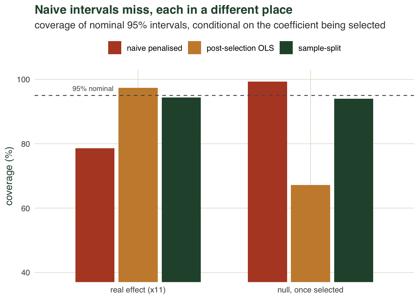
The focal effect is selected in 81 percent of the 2000 datasets. On those datasets, the naive penalised interval covers the true value in only 79 percent, well short of 95. The reason is shrinkage: the penalty pulls the estimate toward zero, so the interval is centred low, at 0.24 on average against a truth of 0.5. Pooled across all the true effects, naive penalised coverage is 58 percent; the stronger the shrinkage relative to the effect, the worse it gets.

Recentring on the refitted least-squares estimate fixes that particular bias: post-selection OLS covers the focal effect 97 percent of the time. It looks valid. It is not, and the null coefficients show where it breaks.

Figure 1: Empirical coverage of nominal 95% intervals, conditional on the coefficient being selected, for the focal real effect and for null coefficients. The naive penalised interval misses the real effect (shrinkage); the post-selection OLS interval misses the nulls (selection); the sample-split interval reaches the line for both.

The winner’s curse

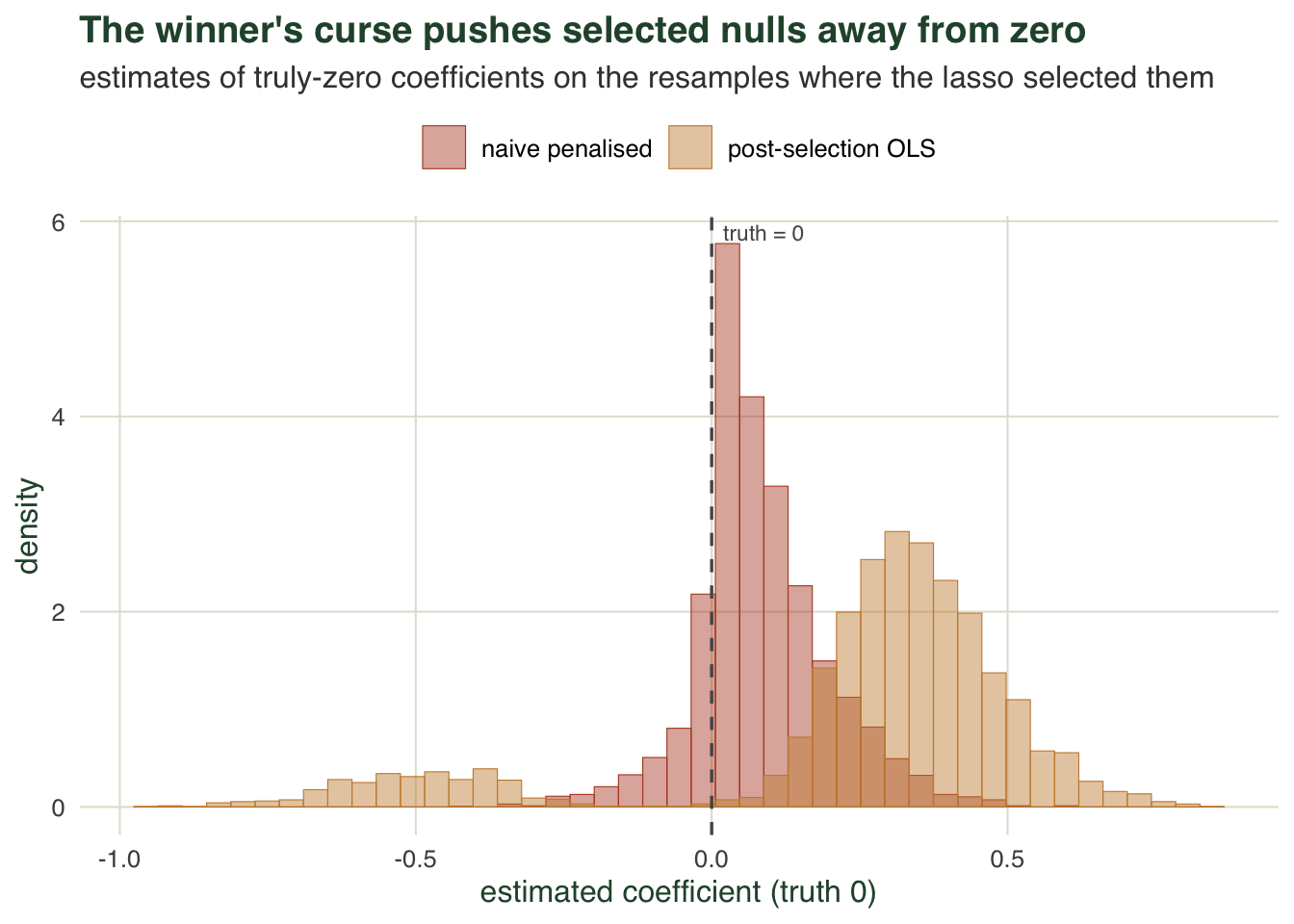
A null predictor is only selected on the datasets where its noise happened to line up with the response. Refit least squares on those datasets and its coefficient is not near zero: selection has already filtered for a large apparent effect. Across the resamples where a null is selected, its post-selection estimate averages 0.24 against a truth of zero, and the naive interval, which knows nothing of the selection, covers zero only 67 percent of the time. The shrinkage that hurt the real effect helps here, pulling the null estimate back toward zero, so the naive penalised interval covers the nulls 99 percent of the time. Neither naive method is valid everywhere: one fails on real effects, the other on nulls.

Figure 2: Estimates of truly-zero coefficients, on the resamples where the lasso selected them. Post-selection least squares pushes them away from zero (the winner’s curse); the penalised estimate stays near zero because the penalty shrinks it back.

What does work

The sample-split interval reaches the nominal line for both the real effect (94 percent) and the nulls (94 percent). The idea is simple: use one half of the data to decide which predictors to look at, and the other, untouched half to estimate and test them. Because the second half played no part in the selection, its ordinary least-squares interval is honest. The cost is power, since each stage sees half the sites, and the selected set is itself noisier on less data. When you cannot spare the sample, resampling the whole pipeline, refitting selection and all on each bootstrap draw, gives the same message from the other direction: it reports how often each predictor is selected and how far its coefficient swings, which is the honest summary when a single interval cannot be trusted. The lasso and elastic net posts used exactly that bootstrap to show selection instability.

The honest limits

Step back to the whole sequence. Ridge, the lasso and the elastic net are different penalties on the same idea, and they share a structure worth stating plainly. The fitted model is a function of three choices the data also drove: the penalty strength, the selection rule, and the cross-validation split. Change the sample a little and the selected set changes, as the bootstrap showed; the surviving coefficients are shrunk, so they are biased as effect sizes; and the interval you would read off the coefficient table is conditioned on a selection event it does not account for. That is why the naive intervals here miss, in two different directions at once.

None of this is an argument against penalised regression. It is an argument about which question it answers. These methods are strong tools for prediction and for screening a long list of candidate predictors down to a plausible few. Read that way, with predictive error quoted from an outer cross-validation and selection stability quoted from a bootstrap, they are honest and useful. Read as a source of effect sizes and confidence intervals, through the ordinary regression table, they are not. If you need valid intervals after selection, hold out data for them by splitting, or use methods built for post-selection inference; do not take the shrunk, selected coefficients at face value.

Related tutorials

• Ridge regression for collinear predictors
• Lasso and variable selection
• Elastic net and cross-validation
• Checking a GAM

References

• Berk, R., Brown, L., Buja, A., Zhang, K. and Zhao, L. 2013. The Annals of Statistics 41(2):802-837 (10.1214/12-AOS1077)
• Lee, J.D., Sun, D.L., Sun, Y. and Taylor, J.E. 2016. The Annals of Statistics 44(3):907-927 (10.1214/15-AOS1371)
• Meinshausen, N. and Buhlmann, P. 2010. Journal of the Royal Statistical Society B 72(4):417-473 (10.1111/j.1467-9868.2010.00740.x)
• Tibshirani, R. 1996. Journal of the Royal Statistical Society B 58(1):267-288 (10.1111/j.2517-6161.1996.tb02080.x)
• Dormann, C.F. et al. 2013. Ecography 36(1):27-46 (10.1111/j.1600-0587.2012.07348.x)
• Hastie, T., Tibshirani, R. and Friedman, J. 2009. The Elements of Statistical Learning, 2nd ed. Springer. ISBN 978-0-387-84857-0