---
title: "Checking a generalised additive model"
description: "Three checks before trusting a fitted GAM: residual autocorrelation that inflates wiggliness, a basis and concurvity screen, and what extrapolation follows."
date: "2026-06-01 15:00"
categories: [GAMs, model checking, diagnostics, ecology tutorial]
image: thumbnail.png
image-alt: "A fitted smooth with a widening confidence band extending beyond the data, diverging from the true curve outside the observed range."
---
A fitted smooth is easy to plot and easy to over-trust. The curve looks reasonable, the confidence band looks tight, and it is tempting to read the wiggles as findings. Three checks stand between a fitted GAM and a defensible conclusion, and each corresponds to a way the fit can mislead: correlated residuals that make the smooth chase noise, a basis or a second smooth that undermines the fit, and extrapolation that reports the shape of the basis rather than the behaviour of the process. This post works through all three on simulated data where the truth is known.
## Check one: residual autocorrelation
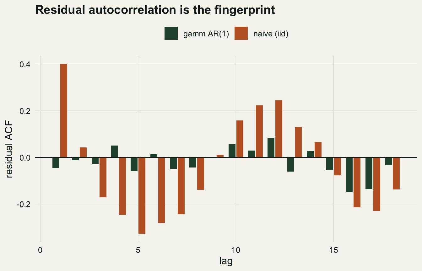
A GAM assumes independent residuals. When the data are a time series or a transect and the residuals are correlated, the smooth mistakes that correlation for signal and bends to follow it, spending far more effective degrees of freedom than the trend warrants. The confidence band tightens at the same time, because the model believes it has more independent information than it does.
```{r}
#| label: setup
#| message: false
#| warning: false
#| code-fold: true
#| code-summary: "Setup: packages, colours and plot theme"
library(mgcv)
library(nlme)
library(ggplot2)
theme_te <- function() {
  theme_minimal(base_size = 12) +
    theme(
      panel.grid.minor = element_blank(),
      panel.grid.major = element_line(colour = "#e5e4dc", linewidth = 0.3),
      plot.background  = element_rect(fill = "#f5f4ee", colour = NA),
      panel.background = element_rect(fill = "#f5f4ee", colour = NA),
      text      = element_text(colour = "#16241d"),
      axis.text = element_text(colour = "#16241d"),
      plot.title = element_text(face = "bold")
    )
}
col_truth <- "#16241d"; col_naive <- "#c0622d"
col_ok    <- "#275139"; col_sage <- "#93a87f"
```
```{r}
#| label: autocorr
#| echo: true
set.seed(4209)
n <- 200; t <- 1:n
mu <- function(t) 3 * sin(pi * t / n)          # gentle single-hump trend
e  <- as.numeric(arima.sim(n = n, list(ar = 0.7), sd = 0.8))
y  <- mu(t) + e
d  <- data.frame(t = t, y = y)

naive <- gam(y ~ s(t, k = 25), data = d, method = "REML")
gmm   <- gamm(y ~ s(t, k = 25), data = d,
              correlation = corAR1(form = ~ t), method = "REML")

p9_edf_naive <- summary(naive)$edf
p9_edf_gamm  <- summary(gmm$gam)$edf
p9_phi       <- as.numeric(coef(gmm$lme$modelStruct$corStruct, unconstrained = FALSE))
p9_acf_naive <- as.numeric(acf(residuals(naive, type = "deviance"),
                               plot = FALSE, lag.max = 1)$acf[2])
p9_acf_gamm  <- as.numeric(acf(residuals(gmm$lme, type = "normalized"),
                               plot = FALSE, lag.max = 1)$acf[2])
p9_ciw_naive <- 2 * 1.96 * predict(naive,     data.frame(t = n/2), se.fit = TRUE)$se.fit
p9_ciw_gamm  <- 2 * 1.96 * predict(gmm$gam,    data.frame(t = n/2), se.fit = TRUE)$se.fit
```
The naive fit, ignoring the correlation, spends `r sprintf("%.1f", p9_edf_naive)` effective degrees of freedom on a trend that is a single smooth hump. Its residuals still carry a lag-one autocorrelation of `r sprintf("%.2f", p9_acf_naive)`: the model has fitted some of the correlated noise and left the rest in the residuals. Adding an AR(1) correlation structure through `gamm` changes the picture entirely. The trend now costs `r sprintf("%.1f", p9_edf_gamm)` degrees of freedom, close to the truth, the estimated autocorrelation is `r sprintf("%.2f", p9_phi)`, recovering the value used to generate the data, and the normalised residuals are white, with a lag-one value of `r sprintf("%.2f", p9_acf_gamm)`. The honest confidence band is wider: at the midpoint it spans `r sprintf("%.2f", p9_ciw_gamm)` against the naive `r sprintf("%.2f", p9_ciw_naive)`.
The residual autocorrelation function is the diagnostic. If it shows structure, the independence assumption has failed, the effective degrees of freedom are inflated, and the intervals are too narrow.
```{r}
#| label: fig-acf
#| echo: false
#| fig-width: 7
#| fig-height: 4.5
#| fig-cap: "Residual autocorrelation before and after modelling the AR(1) structure. The naive fit (orange) leaves correlated residuals; the gamm fit with an AR(1) term (green) whitens them."
#| fig-alt: "A bar-style autocorrelation plot against lag. Orange bars for the naive model show a large positive spike at lag one, then swing between negative and positive values at longer lags; green bars for the AR(1) model stay small at most lags."
al <- 18
an <- acf(residuals(naive, type = "deviance"), plot = FALSE, lag.max = al)
ag <- acf(residuals(gmm$lme, type = "normalized"), plot = FALSE, lag.max = al)
adf <- rbind(
data.frame(lag = 1:al, acf = an$acf[-1], model = "naive (iid)"),
data.frame(lag = 1:al, acf = ag$acf[-1], model = "gamm AR(1)"))
ggplot(adf, aes(lag, acf, fill = model)) +
geom_col(position = position_dodge(width = 0.8), width = 0.7) +
geom_hline(yintercept = 0, colour = col_truth) +
scale_fill_manual(values = c("naive (iid)" = col_naive, "gamm AR(1)" = col_ok)) +
labs(x = "lag", y = "residual ACF", fill = NULL,
title = "Residual autocorrelation is the fingerprint") +
theme_te() +
theme(legend.position = "top")
```
## Check two: basis size and concurvity
Two structural checks come before reading any p-value. The first is whether the basis is large enough, tested with `k.check`; a too-small basis biases the fit, as covered in the companion post on choosing `k`. On a time series, read that post's [section on time as the covariate](../choosing-basis-dimension-k/#when-the-covariate-is-time) before trusting a low k-index. The second is whether smooth terms compete for the same signal, tested with `concurvity`; strong concurvity makes individual smooths and their intervals unreliable, as covered in the post on concurvity.
```{r}
#| label: basis-check
#| echo: true
set.seed(21)
xk <- sort(runif(300))
yk <- sin(2 * pi * xk) + 0.6 * sin(6 * pi * xk) + rnorm(300, 0, 0.3)
m_small <- gam(yk ~ s(xk, k = 5),  method = "REML")
m_big   <- gam(yk ~ s(xk, k = 25), method = "REML")
kc_s <- k.check(m_small); kc_b <- k.check(m_big)
p9_ki5  <- kc_s[1, "k-index"]
p9_ki25 <- kc_b[1, "k-index"]; p9_p25 <- kc_b[1, "p-value"]
```
Here a deliberately small basis fails the check with a k-index of `r sprintf("%.2f", p9_ki5)` and a p-value below 0.001, while the generous basis passes with a k-index of `r sprintf("%.2f", p9_ki25)` and a p-value of `r sprintf("%.2f", p9_p25)`. On the concurvity side, the sibling post builds a case where two smooths have a worst-case concurvity of about 0.91 despite near-zero correlation. Run both checks on any multi-smooth model before interpreting the terms; a clean residual plot does not cover either failure.
## Check three: extrapolation follows the basis
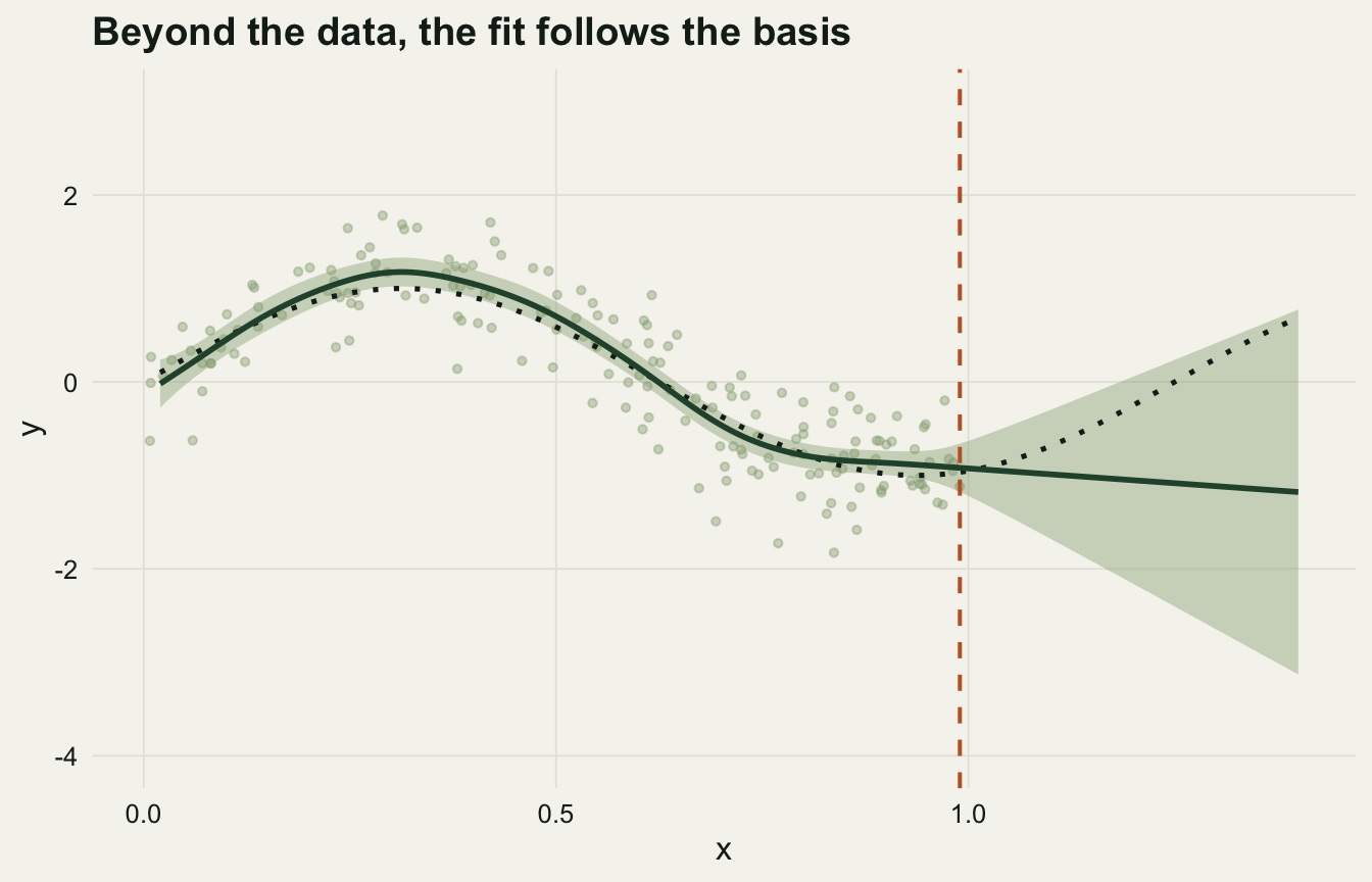
The last check is a caution about the edges. A smooth is supported only within the range of the data. Beyond it, `mgcv` extrapolates according to the boundary behaviour of the basis, which for thin-plate and cubic regression splines is roughly a straight line. The point estimate outside the data is therefore an assumption, not an inference, and the widening confidence band measures uncertainty within that assumption rather than about it.
```{r}
#| label: extrapolation
#| echo: true
set.seed(4219)
xc <- sort(runif(180)); yc <- sin(1.6 * pi * xc) + rnorm(180, 0, 0.4)
dc <- data.frame(x = xc, y = yc)
truef <- function(z) sin(1.6 * pi * z)
m_tp <- gam(y ~ s(x, bs = "tp", k = 15), data = dc, method = "REML")
m_cr <- gam(y ~ s(x, bs = "cr", k = 15), data = dc, method = "REML")

xin <- data.frame(x = seq(0.05, 0.95, length = 60))
p9_in_bases <- max(abs(predict(m_tp, xin) - predict(m_cr, xin)))
p9_in_truth <- sqrt(mean((predict(m_tp, xin) - truef(xin$x))^2))

pe <- predict(m_tp, data.frame(x = 1.30), se.fit = TRUE)
p9_tp13    <- pe$fit
p9_cr13    <- predict(m_cr, data.frame(x = 1.30))
p9_truth13 <- truef(1.30)
p9_lo13    <- pe$fit - 1.96 * pe$se.fit
p9_hi13    <- pe$fit + 1.96 * pe$se.fit
```
Inside the data the two bases are interchangeable: they agree with each other to `r sprintf("%.3f", p9_in_bases)` and track the truth to `r sprintf("%.3f", p9_in_truth)`. Outside the data they still agree with each other, both extrapolating to about `r sprintf("%.2f", p9_tp13)` at `x` of 1.30, so comparing bases would not reveal a problem. But the true curve, a continuing cycle, has turned back up to `r sprintf("%.2f", p9_truth13)`. Both bases are confidently wrong in shape, because both impose a straight-line tail. The interval, `r sprintf("%.2f", p9_lo13)` to `r sprintf("%.2f", p9_hi13)`, happens to contain the truth here, but it is centred on the linear extrapolation the basis assumes; nothing in the observed range constrains the tail, and a periodic or saturating process would leave the band behind.
```{r}
#| label: fig-extrap
#| echo: false
#| fig-width: 7
#| fig-height: 4.5
#| fig-cap: "The fitted smooth (green) with its confidence band, extended beyond the data (vertical line). The band widens but stays centred on a straight-line tail, while the true curve (dotted) turns away. Extrapolation reports the basis, not the process."
#| fig-alt: "A fitted curve with a shaded confidence band over data on the left, continuing past a vertical line marking the edge of the data; beyond that line the band drifts downward in a straight line while the dotted true curve bends upward and climbs to the upper edge of the band without crossing it."
xg <- data.frame(x = seq(0.02, 1.40, length = 200))
pg <- predict(m_tp, xg, se.fit = TRUE)
pdf <- data.frame(x = xg$x, fit = pg$fit, se = pg$se.fit, tru = truef(xg$x))
ggplot(pdf, aes(x)) +
geom_ribbon(aes(ymin = fit - 1.96 * se, ymax = fit + 1.96 * se),
fill = col_sage, alpha = 0.4) +
geom_point(data = dc, aes(x, y), colour = col_sage, alpha = 0.4, size = 1.1) +
geom_line(aes(y = tru), colour = col_truth, linetype = "dotted", linewidth = 0.9) +
geom_line(aes(y = fit), colour = col_ok, linewidth = 1) +
geom_vline(xintercept = max(xc), colour = col_naive, linetype = "dashed", linewidth = 0.7) +
coord_cartesian(ylim = c(-4, 3)) +
labs(x = "covariate x", y = "response y",
title = "Beyond the data, the fit follows the basis") +
theme_te()
```
## The wiggliness is only one sample deep
A closing caution ties the checks together. Even when the residuals are clean, the basis ample, and the range respected, the estimated smoothness is a quantity measured from one dataset, and it varies. Refitting the same process across simulated replicates gives a spread of effective degrees of freedom, not a single number.
```{r}
#| label: edf-spread
#| echo: true
set.seed(303); B <- 400; edfs <- numeric(B)
for (b in 1:B) {
  xb <- sort(runif(180)); yb <- sin(1.6 * pi * xb) + rnorm(180, 0, 0.4)
  edfs[b] <- summary(gam(yb ~ s(xb, k = 15), method = "REML"))$edf
}
p9_edf_med <- median(edfs)
p9_edf_lo  <- quantile(edfs, 0.05); p9_edf_hi <- quantile(edfs, 0.95)
```
The effective degrees of freedom for this fixed process range from `r sprintf("%.1f", p9_edf_lo)` to `r sprintf("%.1f", p9_edf_hi)` across replicates, around a median of `r sprintf("%.1f", p9_edf_med)`. A specific effective degrees of freedom from one fit, and by extension a specific set of wiggles, is an estimate with sampling variability, not a fact about the process. Read a fitted smooth as one draw, check the residuals, the basis, the concurvity and the range, and keep the conclusions inside the data where the model has something to say.
## References
Wood SN 2011. Journal of the Royal Statistical Society Series B 73(1):3-36 (10.1111/j.1467-9868.2010.00749.x).
Augustin NH, Sauleau EA, Wood SN 2012. Computational Statistics and Data Analysis 56(8):2404-2409 (10.1016/j.csda.2012.01.026).
Marra G, Wood SN 2012. Scandinavian Journal of Statistics 39(1):53-74 (10.1111/j.1467-9469.2011.00760.x).
Simpson GL 2018. Frontiers in Ecology and Evolution 6:149 (10.3389/fevo.2018.00149).
Zuur AF, Ieno EN, Walker NJ, Saveliev AA, Smith GM 2009. Mixed Effects Models and Extensions in Ecology with R. Springer. ISBN 978-0-387-87457-9.
Wood SN 2017 Generalized Additive Models: An Introduction with R, 2nd edn, CRC Press, ISBN 978-1-4987-2833-1.
## Related tutorials
- [Choosing a factor smooth for a half-sampled group](../half-sampled-group-in-a-factor-smooth/)
- [Choosing the basis dimension k in mgcv](../choosing-basis-dimension-k/)
- [Concurvity in additive models](../concurvity-in-additive-models/)
- [Overdispersion, year noise and a wiggly GAM trend](../overdispersion-and-a-wiggly-trend/)