---
title: "Penalised regression splines from scratch"
description: "A cubic B-spline basis with a difference penalty, coded by hand and checked against mgcv: the penalty, not the basis degree, decides how wiggly a smooth is."
date: "2026-06-01 12:00"
date-modified: "2026-09-26"
categories: [GAMs, smoothing, regression, ecology tutorial]
image: thumbnail.png
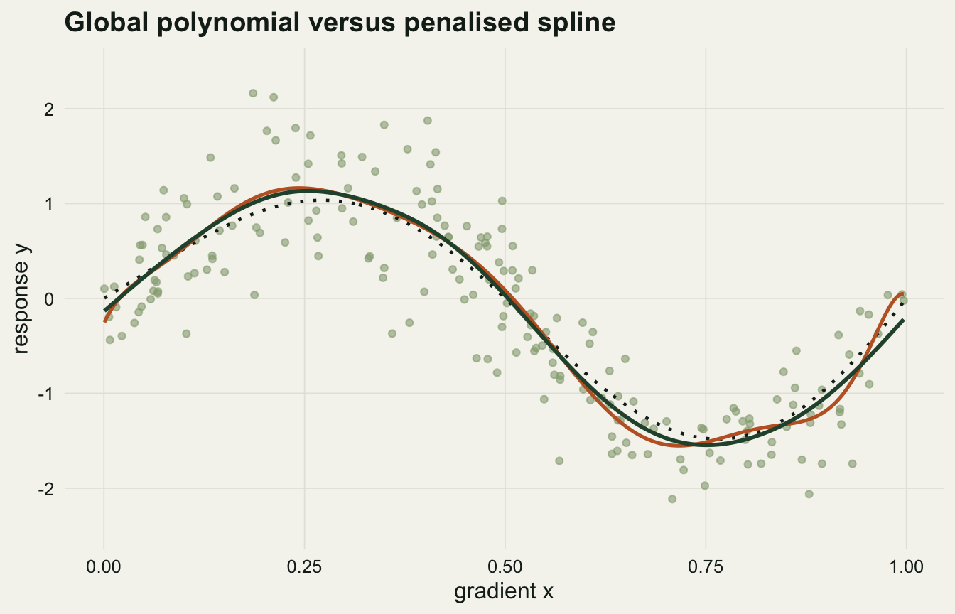
image-alt: "Scatter of points along a gradient with a high-order polynomial in orange and a penalised spline in green, both close to the dotted underlying curve; the polynomial wiggles a little more and dips slightly below it at the left edge."
---
*Updated 26 September 2026: a new section, GCV or REML over many samples, refits both smoothing criteria to fresh samples of this curve and of a straight and an empty term, and measures how often each adds curvature the truth does not have and how much worse than the other each can fit.*
Fitting a smooth curve to an ecological gradient looks like a choice of flexibility: a straight line is too stiff, a high-order polynomial bends to every point. Neither extreme is satisfying. A straight line misses real structure; a flexible polynomial chases noise and behaves wildly near the edges of the data. The usual reflex is to tune the polynomial degree, but degree is a coarse dial, and every step adds global wiggliness that shows up worst where you have least data.
Penalised regression splines take a different route. You lay down a generous set of local basis functions, more than you think you need, and then discourage the fitted coefficients from varying too quickly between neighbours. A single continuous penalty replaces the discrete degree, and the data decide how much of the available flexibility to spend. This post builds the machinery from a B-spline basis and a difference penalty, selects the penalty by generalised cross-validation, and confirms the hand-coded fit against `mgcv::gam`.
## A basis plus a penalty
We simulate a response along a gradient `x` on the unit interval. The truth is a growing-amplitude cycle, smooth but not a polynomial, so a fixed-degree polynomial is always slightly wrong.
```{r}
#| label: setup
#| message: false
#| warning: false
#| code-fold: true
#| code-summary: "Setup: packages, colours and plot theme"
library(splines)
library(mgcv)
library(ggplot2)

theme_te <- function() {
  theme_minimal(base_size = 12) +
    theme(
      panel.grid.minor = element_blank(),
      panel.grid.major = element_line(colour = "#e5e4dc", linewidth = 0.3),
      plot.background  = element_rect(fill = "#f5f4ee", colour = NA),
      panel.background = element_rect(fill = "#f5f4ee", colour = NA),
      text      = element_text(colour = "#16241d"),
      axis.text = element_text(colour = "#16241d"),
      plot.title = element_text(face = "bold")
    )
}
col_truth <- "#16241d"; col_naive <- "#c0622d"
col_pen   <- "#275139"; col_sage  <- "#93a87f"
```
```{r}
#| label: simulate-and-basis
#| echo: true
set.seed(4206)
n <- 200
x <- sort(runif(n))
f <- function(x) sin(2 * pi * x) * (0.8 + 0.9 * x)
sigma <- 0.45
y <- f(x) + rnorm(n, 0, sigma)

## cubic B-spline basis with K functions, equally spaced knots
K <- 20; deg <- 3
rng <- range(x)
nik <- K - deg - 1
dx  <- diff(rng) / (nik + 1)
knots <- c(rng[1] - dx * (deg:1),
           seq(rng[1], rng[2], length = nik + 2),
           rng[2] + dx * (1:deg))
B <- splineDesign(knots, x, ord = deg + 1, outer.ok = TRUE)

## second-order difference penalty on adjacent coefficients
D <- diff(diag(K), differences = 2)
S <- crossprod(D)
```
The basis `B` has `r ncol(B)` columns, one per local bump. The penalty matrix `S` measures how fast the coefficients change from one bump to the next. Fitting minimises the usual residual sum of squares plus a multiple of that roughness, so the smoothing parameter `lambda` trades fit against smoothness continuously.
```{r}
#| label: penalised-fit
#| echo: true
BtB <- crossprod(B); Bty <- crossprod(B, y)
fit_ps <- function(lam) {
  A  <- BtB + lam * S
  Ai <- solve(A)
  beta <- Ai %*% Bty
  fit  <- as.vector(B %*% beta)
  H    <- B %*% Ai %*% t(B)          # influence matrix
  edf  <- sum(diag(H))               # effective degrees of freedom
  rss  <- sum((y - fit)^2)
  gcv  <- n * rss / (n - edf)^2      # generalised cross-validation
  list(beta = beta, fit = fit, edf = edf, gcv = gcv)
}

## select lambda by GCV over a log-spaced grid
lgrid <- 10^seq(-4, 6, length = 200)
gcvv  <- sapply(lgrid, function(l) fit_ps(l)$gcv)
p6_lam    <- lgrid[which.min(gcvv)]
ps_best   <- fit_ps(p6_lam)
ps_unpen  <- fit_ps(1e-8)
p6_edf    <- ps_best$edf
p6_edfun  <- ps_unpen$edf
```
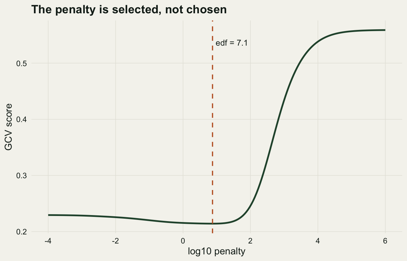
Generalised cross-validation picks a penalty of `r sprintf("%.2f", p6_lam)`. At that penalty the fit spends `r sprintf("%.1f", p6_edf)` effective degrees of freedom, well short of the `r round(p6_edfun)` it would use with the penalty switched off. Effective degrees of freedom count how many free parameters the fit behaves as if it has: the penalty has folded twenty basis functions down to about seven worth of flexibility.
```{r}
#| label: fig-fit
#| echo: false
#| fig-width: 7
#| fig-height: 4.5
#| fig-cap: "A degree-12 polynomial (orange) and the penalised spline (green) against the truth (dotted). Inside the data the two are close, the polynomial drifting furthest at the left edge, by about 0.25. Its real failure sits just outside this window, where it runs to -147 at an x of 1.15."
#| fig-alt: "Scatter plot of the simulated data with three curves: a dotted line for the true function, an orange polynomial curve that follows it closely except at the left edge where it dips about a quarter of a unit below, and a green penalised-spline curve that stays close to the dotted line throughout."
poly12 <- lm(y ~ poly(x, 12))
grid <- data.frame(x = seq(min(x), max(x), length = 400))
Bg <- splineDesign(knots, grid$x, ord = deg + 1, outer.ok = TRUE)
grid$pen <- as.vector(Bg %*% ps_best$beta)
grid$pl12 <- predict(poly12, grid)
grid$tru <- f(grid$x)
ggplot() +
geom_point(data = data.frame(x, y), aes(x, y),
colour = col_sage, alpha = 0.6, size = 1.4) +
geom_line(data = grid, aes(x, tru), colour = col_truth,
linetype = "dotted", linewidth = 0.8) +
geom_line(data = grid, aes(x, pl12), colour = col_naive, linewidth = 0.9) +
geom_line(data = grid, aes(x, pen), colour = col_pen, linewidth = 1) +
coord_cartesian(ylim = c(-2.4, 2.4)) +
labs(x = "gradient x", y = "response y",
title = "Global polynomial versus penalised spline") +
theme_te()
```
## Does the hand-coded fit match mgcv?
The point of coding the penalty by hand is to see that nothing is hidden. To check it, we fit the same P-spline through `mgcv`, which places the knots slightly differently and applies its own identifiability constraint, then compare fitted values.
```{r}
#| label: mgcv-check
#| echo: true
d <- data.frame(x = x, y = y)
m_gcv  <- gam(y ~ s(x, bs = "ps", k = 20, m = c(2, 2)), data = d, method = "GCV.Cp")
m_reml <- gam(y ~ s(x, bs = "ps", k = 20, m = c(2, 2)), data = d, method = "REML")

p6_edfmg   <- sum(m_gcv$edf)                 # total, including intercept
p6_edfsm   <- summary(m_gcv)$edf             # smooth term only, GCV
p6_edfreml <- summary(m_reml)$edf            # smooth term only, REML
p6_maxdiff <- max(abs(ps_best$fit - as.vector(predict(m_gcv))))
```
The two fits agree to `r sprintf("%.4f", p6_maxdiff)` at every point: the hand-coded total of `r sprintf("%.1f", p6_edf)` effective degrees of freedom sits alongside mgcv's `r sprintf("%.1f", p6_edfmg)`, both counts including the intercept. Compare the smooth term on its own and the criteria separate: `r sprintf("%.1f", p6_edfsm)` degrees of freedom under generalised cross-validation against `r sprintf("%.1f", p6_edfreml)` under restricted maximum likelihood, the selection Wood (2011) recommends because its criterion has a better defined optimum. On this sample REML smooths a little less, not more. The machinery is the same either way; only the criterion for `lambda` differs.
## GCV or REML over many samples
The comparison above rests on one sample, and `gam()` does not ask which criterion you want: without a `method` argument it uses generalised cross-validation, `method = "GCV.Cp"` in mgcv `r packageDescription("mgcv")$Version`, the version this post was knitted with (the chunk below stops if a later version changes the default). To see whether "REML smooths a little less" belongs to the criterion or to this draw, the chunk refits both criteria to 400 fresh samples of the same curve, with the same `n`, noise standard deviation and P-spline basis. A second arm fits `y ~ s(x) + s(z)` to data in which `x` has a straight effect of slope 1.5 and `z` has none, the same basis for both terms. The second-order difference penalty leaves a straight line unpenalised, so a term fitted as a line has about one effective degree of freedom, and more than two means curvature the truth does not have.
```{r}
#| label: criteria-sim
#| echo: true
stopifnot(identical(formals(gam)$method, "GCV.Cp"),   # the default measured here,
          gam(round(3 * exp(f(x))) ~ s(x), family = poisson)$method == "UBRE")  # UBRE for counts
crit_reps <- 400; crit_slope <- 1.5
crit_ps <- function(v) sprintf("s(%s, bs = 'ps', k = 20, m = c(2, 2))", v)
crit_pair <- function(fm, dat) list(g = gam(fm, data = dat, method = "GCV.Cp"),
                                    r = gam(fm, data = dat, method = "REML"))
crit_wiggly <- function() {                 # this post's curve, n and sigma
  dw <- data.frame(xw = sort(runif(n))); dw$yw <- f(dw$xw) + rnorm(n, 0, sigma)
  fp <- crit_pair(as.formula(paste("yw ~", crit_ps("xw"))), dw)
  c(edf_g = summary(fp$g)$edf, edf_r = summary(fp$r)$edf,
    rmse_g = sqrt(mean((fitted(fp$g) - f(dw$xw))^2)),
    rmse_r = sqrt(mean((fitted(fp$r) - f(dw$xw))^2)))
}
crit_straight <- function() {               # x straight, z no effect at all
  ds <- data.frame(xs = runif(n), zs = runif(n))
  ds$ys <- crit_slope * ds$xs + rnorm(n, 0, sigma)
  fp <- crit_pair(as.formula(paste("ys ~", crit_ps("xs"), "+", crit_ps("zs"))), ds)
  sg <- summary(fp$g)$s.table; sr <- summary(fp$r)$s.table
  c(lin_g = sg[1, "edf"], lin_r = sr[1, "edf"], nul_g = sg[2, "edf"],
    nul_r = sr[2, "edf"], p_g = sg[2, "p-value"], p_r = sr[2, "p-value"])
}
set.seed(14302)
crit_w <- as.data.frame(t(replicate(crit_reps, crit_wiggly())))
crit_s <- as.data.frame(t(replicate(crit_reps, crit_straight())))
## share of samples, with its Monte Carlo standard error
crit_share <- function(v) c(p = mean(v), se = sqrt(mean(v) * (1 - mean(v)) / length(v)))
crit_lin <- sapply(crit_s[c("lin_g", "lin_r")], function(e) crit_share(e > 2))
crit_nul <- sapply(crit_s[c("nul_g", "nul_r")], function(e) crit_share(e > 2))
crit_fp  <- sapply(crit_s[c("p_g", "p_r")], function(p) crit_share(p < 0.05))
crit_q95 <- sapply(crit_s[c("nul_g", "nul_r")], quantile, probs = 0.95)
crit_more <- crit_share(crit_w$edf_r > crit_w$edf_g)
crit_qw <- sapply(crit_w[c("edf_g", "edf_r")], quantile, probs = c(0.05, 0.5, 0.95))
crit_ratio <- crit_w$rmse_g / crit_w$rmse_r
crit_bad_g <- crit_share(crit_ratio > 1.25); crit_bad_r <- crit_share(crit_ratio < 0.8)
crit_bad_up <- (crit_w$edf_g > crit_w$edf_r)[crit_ratio > 1.25]
```
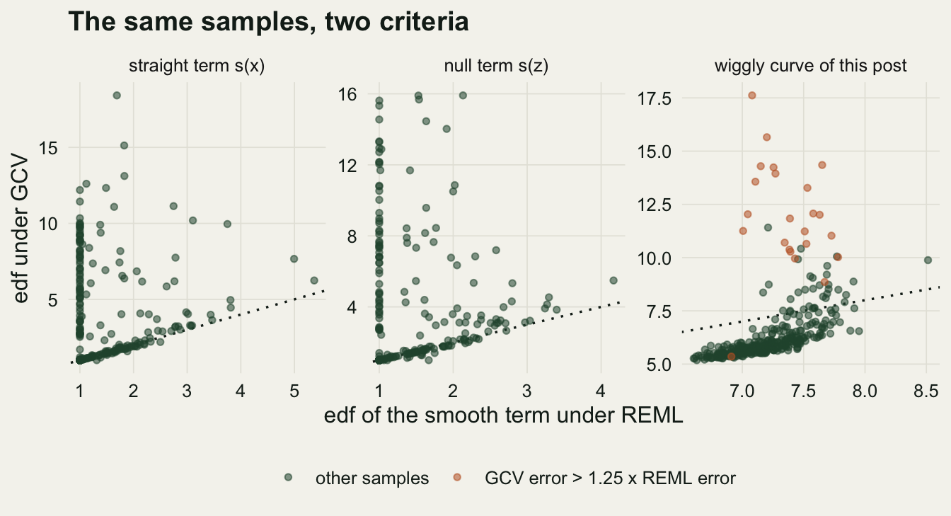
On the straight term GCV spends more than two effective degrees of freedom in `r sprintf("%.3f", crit_lin["p", "lin_g"])` of samples and REML in `r sprintf("%.3f", crit_lin["p", "lin_r"])`; on the null term the shares are `r sprintf("%.3f", crit_nul["p", "nul_g"])` and `r sprintf("%.3f", crit_nul["p", "nul_r"])` (Monte Carlo standard errors between `r sprintf("%.3f", min(crit_lin["se", ], crit_nul["se", ]))` and `r sprintf("%.3f", max(crit_lin["se", ], crit_nul["se", ]))`), so GCV bends a term that is straight or empty about three times as often as REML (the ratios of the two shares are `r sprintf("%.1f", crit_lin["p", "lin_g"] / crit_lin["p", "lin_r"])` and `r sprintf("%.1f", crit_nul["p", "nul_g"] / crit_nul["p", "nul_r"])`). Its tail is long: the 95th percentile, over samples, of the null term's effective degrees of freedom is `r sprintf("%.1f", crit_q95[["nul_g.95%"]])` under GCV and `r sprintf("%.1f", crit_q95[["nul_r.95%"]])` under REML. The p-values barely notice. The null term is called significant at 5 per cent in `r sprintf("%.3f", crit_fp["p", "p_g"])` of samples under GCV and `r sprintf("%.3f", crit_fp["p", "p_r"])` under REML, each with a standard error of about `r sprintf("%.3f", crit_fp["se", "p_g"])`.
On this post's wiggly curve the usual sample goes the other way. REML spends more degrees of freedom than GCV in `r sprintf("%.3f", crit_more[["p"]])` of samples (standard error `r sprintf("%.3f", crit_more[["se"]])`), so the sample above, where REML smoothed a little less, was the usual case. The median smooth-term edf is `r sprintf("%.1f", crit_qw["50%", "edf_g"])` under GCV and `r sprintf("%.1f", crit_qw["50%", "edf_r"])` under REML; GCV's 5th to 95th percentile runs from `r sprintf("%.1f", crit_qw["5%", "edf_g"])` to `r sprintf("%.1f", crit_qw["95%", "edf_g"])`, REML's from `r sprintf("%.1f", crit_qw["5%", "edf_r"])` to `r sprintf("%.1f", crit_qw["95%", "edf_r"])`. Accuracy against the truth is almost level: mean root mean squared error `r sprintf("%.4f", mean(crit_w$rmse_g))` for GCV and `r sprintf("%.4f", mean(crit_w$rmse_r))` for REML, and a median ratio of GCV error to REML error of `r sprintf("%.2f", median(crit_ratio))`. The price of GCV's spread is a tail, and what sets it apart is how far the tail reaches more than how often it is hit. In `r sprintf("%.3f", crit_bad_g[["p"]])` of samples (standard error `r sprintf("%.3f", crit_bad_g[["se"]])`) its error is more than 1.25 times REML's, and in `r sprintf("%d", sum(crit_bad_up))` of those `r sprintf("%d", sum(crit_ratio > 1.25))` samples GCV had spent more degrees of freedom than REML: the kind of failure Wood (2011) describes, a small number of severe undersmoothing fits under GCV. REML's error exceeds 1.25 times GCV's in `r sprintf("%.3f", crit_bad_r[["p"]])` of samples (standard error `r sprintf("%.3f", crit_bad_r[["se"]])`), but never by much: its worst sample is `r sprintf("%.2f", max(1 / crit_ratio))` times GCV's error, while GCV's error is more than 1.5 times REML's in `r sprintf("%d", sum(crit_ratio > 1.5))` of the `r sprintf("%d", crit_reps)` samples and reaches `r sprintf("%.1f", max(crit_ratio))` times.
```{r}
#| label: fig-criteria
#| echo: false
#| fig-width: 7
#| fig-height: 3.8
#| fig-cap: "Effective degrees of freedom of the smooth term under GCV against REML, one point per simulated sample and both criteria fitted to the same data. The dotted line marks equal edf. In the right panel, orange marks samples in which the GCV fit's error against the truth is more than 1.25 times the REML fit's."
#| fig-alt: "Three scatter panels on off-white paper, each plotting the effective degrees of freedom under GCV on the vertical axis against those under REML on the horizontal axis, with a dotted line of equal values. In the straight-term panel most points lie on the line between 1 and 2, but a column of points at a REML value of 1 rises to GCV values near 10, a few of them to 12, scattered points beside it reach 13 and 15, and one point reaches about 18. The null-term panel shows the same pattern: a dense cluster at 1 and 1, a column at a REML value of 1 reaching GCV values near 16, and scattered points above the line. In the wiggly-curve panel REML values run from about 6.6 to 8.5, most points sit below the dotted line at GCV values between 5 and 7.5, and 22 orange points lie above it at GCV values from about 9 to 17.6, most above 10, with one orange point below the line near the bottom. A legend at the bottom names the green points other samples and the orange points GCV error above 1.25 times REML error."
crit_arms <- c("straight term s(x)", "null term s(z)", "wiggly curve of this post")
crit_pts <- data.frame(arm = factor(rep(crit_arms, each = crit_reps), levels = crit_arms),
reml = c(crit_s$lin_r, crit_s$nul_r, crit_w$edf_r),
gcv = c(crit_s$lin_g, crit_s$nul_g, crit_w$edf_g),
bad = c(rep(FALSE, 2 * crit_reps), crit_ratio > 1.25))
ggplot(crit_pts[order(crit_pts$bad), ], aes(reml, gcv)) +
geom_abline(intercept = 0, slope = 1, colour = col_truth, linetype = "dotted", linewidth = 0.6) +
geom_point(aes(colour = bad), alpha = 0.55, size = 1.3) +
scale_colour_manual(values = c(`FALSE` = col_pen, `TRUE` = col_naive), name = NULL,
labels = c("other samples", "GCV error > 1.25 x REML error")) +
facet_wrap(~ arm, scales = "free") +
labs(x = "edf of the smooth term under REML", y = "edf under GCV", title = "The same samples, two criteria") +
theme_te() + theme(legend.position = "bottom")
```
GCV's fault here is spread, not a consistent direction: it adds curvature to straight and empty terms far more often than REML, and on a curve that really bends it usually smooths more than REML, in exchange for a handful of fits much worse than REML's on the same data, while REML is never much worse than GCV. Neither criterion smooths more on every curve. On a narrow seasonal pulse in [Harmonics or cyclic splines for a narrow seasonal peak](../cyclic-splines-for-seasonal-data/) the typical fit runs the other way, REML smoothing more than UBRE (what `method = "GCV.Cp"` uses for Poisson counts, where the scale is known) and widening the crest, while UBRE's occasional runaway spike is the same kind of tail. What `method = "REML"` buys is a steadier choice of penalty, not a smoother or rougher curve; since it is not the default, it has to be written in the call. This is one sample size, one noise level, one basis (a 20-function P-spline) and a Gaussian response.
## Too stiff, too flexible, or penalised
The three fitting strategies fail and succeed in instructive ways. We compare each against the known truth by root mean squared error, and we ask what each does just outside the data, at `x` equal to 1.15.
```{r}
#| label: compare
#| echo: true
poly4 <- lm(y ~ poly(x, 4)); poly12 <- lm(y ~ poly(x, 12))
truef <- f(x)
rmse  <- function(fit) sqrt(mean((fit - truef)^2))

p6_r_p4  <- rmse(fitted(poly4))
p6_r_p12 <- rmse(fitted(poly12))
p6_r_un  <- rmse(ps_unpen$fit)
p6_r_pen <- rmse(ps_best$fit)

xe <- 1.15
Be <- splineDesign(knots, xe, ord = deg + 1, outer.ok = TRUE)
p6_ext_pen <- as.vector(Be %*% ps_best$beta)
p6_ext_p12 <- as.vector(predict(poly12, data.frame(x = xe)))

## how much basis is left at and beyond the edge of the data
p6_row_in  <- sum(splineDesign(knots, max(x), ord = deg + 1, outer.ok = TRUE))
p6_row_mid <- sum(splineDesign(knots, 1.05,   ord = deg + 1, outer.ok = TRUE))
p6_row_out <- sum(Be)
```
Against the truth, the penalised spline reaches an error of `r sprintf("%.3f", p6_r_pen)`, beating both the low-order polynomial (`r sprintf("%.3f", p6_r_p4)`) and the unpenalised spline (`r sprintf("%.3f", p6_r_un)`). The ranking is the whole story in miniature. The degree-4 polynomial is too stiff and misses the shape; the unpenalised spline is too flexible and fits the noise; the penalty lands between them without anyone choosing where. The high-order polynomial is worst of all outside the data: at `x` of 1.15 it predicts `r sprintf("%.0f", p6_ext_p12)`, a runaway swing, while the spline stays bounded and returns `r sprintf("%.2f", p6_ext_pen)`. Bounded is not the same as right, since the truth there is `r sprintf("%.2f", f(xe))`, and the next section says where that zero comes from.
```{r}
#| label: fig-gcv
#| echo: false
#| fig-width: 7
#| fig-height: 4.5
#| fig-cap: "The generalised cross-validation score as a function of the penalty. The minimum (marked) selects the smoothing parameter; nobody sets the wiggliness by hand."
#| fig-alt: "A U-shaped curve of the GCV score against the log penalty, with a vertical dashed line marking the minimum near a penalty of about seven, annotated with the effective degrees of freedom at that point."
gdf <- data.frame(loglam = log10(lgrid), gcv = gcvv)
ggplot(gdf, aes(loglam, gcv)) +
geom_line(colour = col_pen, linewidth = 1) +
geom_vline(xintercept = log10(p6_lam), linetype = "dashed",
colour = col_naive, linewidth = 0.7) +
annotate("text", x = log10(p6_lam), y = max(gcvv) * 0.96,
label = sprintf("edf = %.1f", p6_edf), hjust = -0.1,
colour = col_truth, size = 3.6) +
labs(x = "log10 penalty", y = "GCV score",
title = "The penalty is selected, not chosen") +
theme_te()
```
## What the penalty does and does not buy
The penalty turns a discrete modelling decision into an estimated quantity. You no longer commit to a degree; you provide enough basis functions and let generalised cross-validation or restricted maximum likelihood set the effective flexibility. That removes the worst failure of global polynomials, the wild boundary behaviour, and it adapts the fit to the data at hand.
It does not make extrapolation safe. The penalised spline stayed bounded outside the data, but bounded here means dead. A B-spline basis sums to one only across the interval its knots cover; past the last data knot the bumps run out one by one, so the design row that sums to `r sprintf("%.2f", p6_row_in)` at the edge of the data sums to `r sprintf("%.2f", p6_row_mid)` at an `x` of 1.05 and `r sprintf("%.2f", p6_row_out)` at 1.15. The fit is dragged to zero, which is why it returned `r sprintf("%.2f", p6_ext_pen)` against a true `r sprintf("%.2f", f(xe))`. That is the basis ending rather than any statement about the process. The penalty controls behaviour inside the data, where there is information; outside, the fit follows the basis. Nothing here tells you how the curve behaves where you have no points, and the smoothness itself is only weakly identified from a single sample. Those limits are the subject of the rest of this cluster: how large the basis should be, what goes wrong when smooth terms compete for the same signal, and how to check a fitted smooth before trusting it.
## References
Eilers PHC, Marx BD 1996. Statistical Science 11(2):89-121 (10.1214/ss/1038425655).
Hastie T, Tibshirani R 1986. Statistical Science 1(3):297-310 (10.1214/ss/1177013604).
Craven P, Wahba G 1979. Numerische Mathematik 31(4):377-403 (10.1007/BF01404567).
Wood SN 2011. Journal of the Royal Statistical Society Series B 73(1):3-36 (10.1111/j.1467-9868.2010.00749.x).
Wood SN 2017 Generalized Additive Models: An Introduction with R, 2nd edn, CRC Press, ISBN 978-1-4987-2833-1.
## Related tutorials
- [Choosing the basis dimension k in mgcv](../choosing-basis-dimension-k/)
- [Concurvity in additive models](../concurvity-in-additive-models/)
- [Checking a generalised additive model](../checking-a-gam/)
- [Tensor product smooths in mgcv](../tensor-product-smooths-in-mgcv/)