---
title: "Choosing the basis dimension k in mgcv"
description: "The k in a GAM smooth is a ceiling on wiggliness, not the fit. Set it generously, let the penalty work, and check with k.check that the basis is large enough."
date: "2026-06-01 13:00"
date-modified: "2026-09-27"
categories: [GAMs, smoothing, model selection, ecology tutorial]
image: thumbnail.png
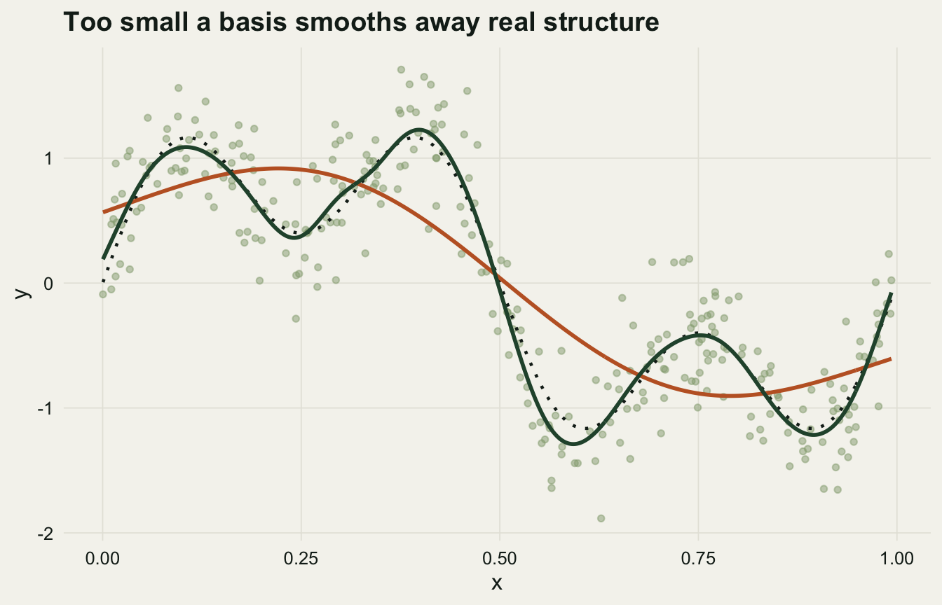
image-alt: "A single panel of pale green points scattered around a black dotted true curve, with a dark green fit that follows every wiggle and a smooth orange fit that keeps only the broad rise and fall because its basis dimension is too small."
---
*Updated 27 September 2026: a new section, When the covariate is time, shows that the k-index is a Durbin-Watson statistic along the covariate, so errors correlated in time flag a smooth of time at any basis size tried here while raising k fits part of the noise, and the rule in Setting k in practice now points to it.*
Every `s(x)` in an `mgcv` model carries a `k`, the basis dimension, and it invites a familiar worry: what if I pick it wrong? The worry is misplaced, because `k` does not set how wiggly the fitted smooth is. The penalty does that. What `k` sets is a ceiling: the most wiggliness the smooth is allowed to reach. Provided the ceiling is high enough to contain the structure in the data, the penalty pulls the effective flexibility down to whatever the data support, and the exact value of `k` above that point barely matters.
This is the same idea as mesh convergence in a numerical solver. You refine the grid until the answer stops moving, then stop worrying about the grid. Here you raise `k` until the fit stops changing, confirm the basis is not the limiting factor, and move on. This post shows the ceiling in action and demonstrates the `k.check` diagnostic that tells you when the ceiling is too low.
## A fit that needs some wiggliness
The truth combines a slow cycle with a faster ripple, so it needs a fair amount of flexibility to represent, roughly sixteen effective degrees of freedom. We fit the same smooth at a ladder of `k` values and record two things: the effective degrees of freedom the penalty settles on, and how close the fit gets to the known truth.
```{r}
#| label: setup
#| message: false
#| warning: false
#| code-fold: true
#| code-summary: "Setup: packages, colours and plot theme"
library(mgcv)
library(ggplot2)
theme_te <- function() {
  theme_minimal(base_size = 12) +
    theme(
      panel.grid.minor = element_blank(),
      panel.grid.major = element_line(colour = "#e5e4dc", linewidth = 0.3),
      plot.background  = element_rect(fill = "#f5f4ee", colour = NA),
      panel.background = element_rect(fill = "#f5f4ee", colour = NA),
      strip.text = element_text(colour = "#16241d", face = "bold"),
      text      = element_text(colour = "#16241d"),
      axis.text = element_text(colour = "#16241d"),
      plot.title = element_text(face = "bold")
    )
}
col_truth <- "#16241d"; col_low <- "#c0622d"
col_ok    <- "#275139"; col_sage <- "#93a87f"
```
```{r}
#| label: k-ladder
#| echo: true
set.seed(4207)
n <- 300
x <- sort(runif(n))
f <- function(x) sin(2 * pi * x) + 0.6 * sin(6 * pi * x)
sigma <- 0.3
y <- f(x) + rnorm(n, 0, sigma)
d <- data.frame(x = x, y = y)
truef <- f(x)
rmse  <- function(fit) sqrt(mean((fit - truef)^2))

ks <- c(4, 6, 8, 12, 16, 24, 32)
res <- lapply(ks, function(k) {
  m  <- gam(y ~ s(x, bs = "tp", k = k), data = d, method = "REML")
  kc <- k.check(m)
  data.frame(k = k, edf = summary(m)$edf, rmse = rmse(fitted(m)),
             ceiling = k - 1, kindex = kc[1, "k-index"], kp = kc[1, "p-value"])
})
res <- do.call(rbind, res)
```
```{r}
#| label: pull-numbers
#| echo: false
g <- function(kk, col) res[[col]][res$k == kk]
p7_edf4 <- g(4,"edf"); p7_rmse4 <- g(4,"rmse"); p7_ki4 <- g(4,"kindex")
p7_edf8 <- g(8,"edf"); p7_rmse8 <- g(8,"rmse"); p7_ki8 <- g(8,"kindex"); p7_p8 <- g(8,"kp")
p7_edf24 <- g(24,"edf"); p7_rmse24<- g(24,"rmse"); p7_ki24 <- g(24,"kindex"); p7_p24<- g(24,"kp")
p7_edf32 <- g(32,"edf"); p7_rmse32<- g(32,"rmse")
```
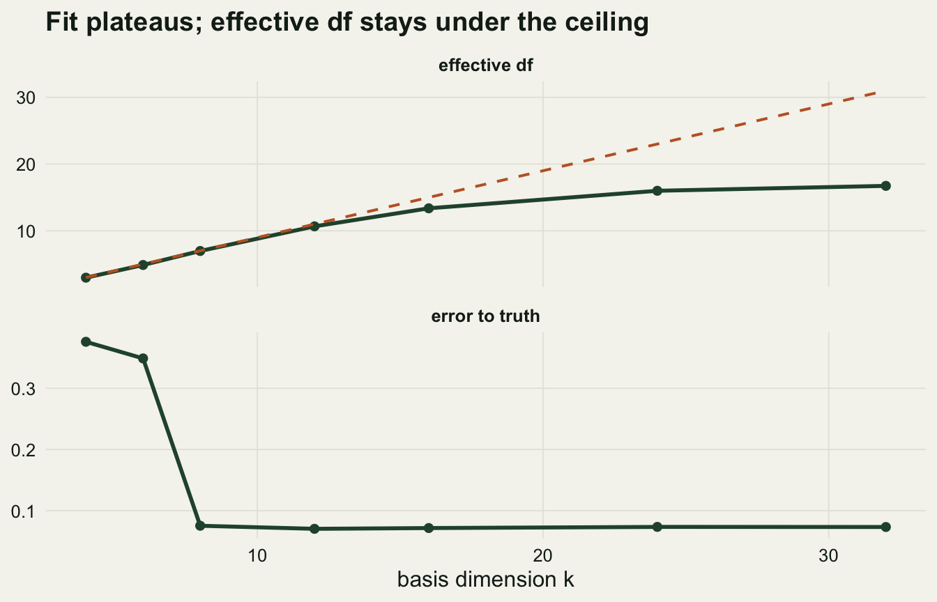
At `k` equal to 4 the basis is too small to hold the ripple. The fit uses `r sprintf("%.1f", p7_edf4)` effective degrees of freedom (near its ceiling of three) and lands `r sprintf("%.3f", p7_rmse4)` from the truth. By `k` equal to 8 the error has dropped to `r sprintf("%.3f", p7_rmse8)` and stays there: at `k` of 24 it is `r sprintf("%.3f", p7_rmse24)`, and at `k` of 32 it is `r sprintf("%.3f", p7_rmse32)`. Adding basis functions past the point of sufficiency does not change the fit, because the penalty absorbs them.
The effective degrees of freedom tell the complementary story. They keep climbing, from `r sprintf("%.1f", p7_edf8)` at `k` of 8 to `r sprintf("%.1f", p7_edf24)` at 24 and `r sprintf("%.1f", p7_edf32)` at 32, but the growth decelerates and stays far below the ceiling of `r round(res$ceiling[res$k==32])`. The gap between the effective degrees of freedom and the ceiling widens as `k` grows: that gap is the penalty working harder to hold the extra flexibility in check.
```{r}
#| label: fig-fits
#| fig-width: 7
#| fig-height: 4.5
#| fig-cap: "At k equal to 4 (orange) the basis cannot represent the ripple and the fit is smoothed past the real structure. At k equal to 24 (green) the fit recovers the truth (dotted). More basis functions do not overfit; the penalty holds them back."
#| fig-alt: "Scatter of points with three curves: a dotted true curve with a clear ripple, an orange curve at low k that misses the ripple entirely, and a green curve at high k that follows the ripple closely."
#| code-fold: true
#| code-summary: "Show the code behind this output"
m4  <- gam(y ~ s(x, bs = "tp", k = 4),  data = d, method = "REML")
m24 <- gam(y ~ s(x, bs = "tp", k = 24), data = d, method = "REML")
gr <- data.frame(x = seq(min(x), max(x), length = 400))
gr$k4  <- predict(m4,  gr); gr$k24 <- predict(m24, gr); gr$tru <- f(gr$x)
ggplot() +
  geom_point(data = d, aes(x, y), colour = col_sage, alpha = 0.5, size = 1.3) +
  geom_line(data = gr, aes(x, tru), colour = col_truth, linetype = "dotted", linewidth = 0.8) +
  geom_line(data = gr, aes(x, k4),  colour = col_low, linewidth = 1) +
  geom_line(data = gr, aes(x, k24), colour = col_ok,  linewidth = 1) +
  labs(x = "x", y = "y", title = "Too small a basis smooths away real structure") +
  theme_te()
```
## The k.check diagnostic
If the fit is insensitive to `k` once the basis is large enough, how do you know you have cleared that threshold? You check whether the residuals still carry pattern the smooth could not reach. The `k.check` function in `mgcv` does this by ordering the residuals along the covariate and comparing the variance of differences between neighbours to the overall residual variance. If the basis was too small, neighbouring residuals stay on the same side of zero across the stretch the smooth missed, so their differences are unusually small and the ratio, the k-index, falls below one.
```{r}
#| label: hand-kindex
#| echo: true
hand_kindex <- function(m) {
  e  <- residuals(m, type = "deviance")
  eo <- e[order(d$x)]
  mean(diff(eo)^2) / (2 * var(e))
}
p7_hk4  <- hand_kindex(m4)
p7_hk24 <- hand_kindex(m24)
```
The hand version captures the principle: the neighbour-difference index is `r sprintf("%.2f", p7_hk4)` at `k` of 4 and `r sprintf("%.2f", p7_hk24)` at `k` of 24, below one where structure remains and near one where it does not. The `k.check` implementation refines this and adds a permutation p-value, which is the number to read in practice. It flags `k` of 4 firmly, with a k-index of `r sprintf("%.2f", p7_ki4)` and a p-value below 0.001, and clears `k` of 8, with a k-index of `r sprintf("%.2f", p7_ki8)` and a p-value of `r sprintf("%.2f", p7_p8)`. At `k` of 24 the k-index is `r sprintf("%.2f", p7_ki24)`, clear. A low k-index with a small p-value is the signal to raise `k` and refit.
```{r}
#| label: fig-plateau
#| echo: false
#| fig-width: 7
#| fig-height: 4.5
#| fig-cap: "Error against basis dimension falls sharply and then plateaus; effective degrees of freedom climb, sitting on the k minus 1 ceiling (dashed) while the basis is too small and pulling away from it once k is large enough. Beyond the threshold, k costs computation, not accuracy."
#| fig-alt: "Two stacked panels against k on the x axis: the top panel shows effective degrees of freedom rising and levelling off, with a dashed k minus 1 ceiling that runs along them at small k and climbs away above them at large k; the bottom panel shows RMSE dropping steeply then flattening near a low value."
long <- rbind(
data.frame(k = res$k, value = res$rmse, panel = "error to truth"),
data.frame(k = res$k, value = res$edf, panel = "effective df"))
ceil <- data.frame(k = res$k, value = res$ceiling, panel = "effective df")
ggplot(long, aes(k, value)) +
geom_line(colour = col_ok, linewidth = 1) +
geom_point(colour = col_ok, size = 1.8) +
geom_line(data = ceil, aes(k, value), colour = col_low,
linetype = "dashed", linewidth = 0.7) +
facet_wrap(~panel, ncol = 1, scales = "free_y") +
labs(x = "basis dimension k", y = NULL,
title = "Fit plateaus; effective df stays under the ceiling") +
theme_te()
```
## Setting k in practice
The practical rule follows from the ceiling picture. Start `k` generously, larger than you expect the effective degrees of freedom to be, and let restricted maximum likelihood set the smoothness. Run `k.check`. If a smooth shows a low k-index and a small p-value, its basis is usually the binding constraint, so raise its `k` and refit; when the covariate is time or position along a transect, read the section below first. If the check is clear, the basis is not limiting the fit and there is nothing to tune.
Two limits are worth stating plainly. The check is a guide, not a guarantee: it detects leftover pattern along the covariate, and a basis that misses structure in some other way can still pass. And the true wiggliness is never known; `k` only needs to exceed the effective degrees of freedom the data can support, which is itself an estimate from one sample. Raising `k` past the plateau is cheap insurance against the first problem and costs only computation. Under-setting it is the error that biases the fit, as the `k` equal to 4 curve showed.
## When the covariate is time
The k-index has a name outside `mgcv`. The sum of squared differences between neighbouring residuals, divided by the sum of squared residuals, is the Durbin-Watson statistic for serial correlation (Durbin and Watson 1950), taken here along the covariate instead of along time. The `k.check` source averages the n minus 1 differences and the n squared residuals, so its k-index is half the Durbin-Watson statistic times n/(n minus 1), a factor of `r sprintf("%.3f", n / (n - 1))` at 300 points; the hand version above is exactly half the statistic. The Durbin-Watson statistic is close to two times one minus the lag-one correlation of the residuals, so the k-index reads as one minus that correlation along the covariate. When the covariate is the sampling date (or position along a transect) and the errors carry over from one visit, or one station, to the next, a low k-index follows from that definition whether or not the basis is large enough. To see what that does to the rule above, the chunk reads `x` as the date of each visit in one season and gives the errors a lag-one (AR(1)) correlation `phi` between successive visits, keeping the post's error standard deviation. A second arm keeps the same correlated errors in visit order but uses a covariate drawn at random for each visit, unrelated to its date, so its order says nothing about time. Each cell is 60 simulated seasons, and a fit counts as flagged when the k-index is below one with a p-value below 0.05.
```{r}
#| label: time-covariate
#| echo: true
set.seed(2609)
tk_fit <- function(phi, k, in_time) {
  e  <- if (phi == 0) rnorm(n, 0, sigma) else
    as.numeric(arima.sim(list(ar = phi), n, sd = sigma * sqrt(1 - phi^2)))
  xs <- if (in_time) sort(runif(n)) else runif(n)  # rows stay in visit order
  ys <- f(xs) + e; m <- gam(ys ~ s(xs, bs = "tp", k = k), method = "REML")
  kc <- k.check(m); r <- residuals(m); ro <- r[order(xs)]
  c(flag = kc[1, "k-index"] < 1 && kc[1, "p-value"] < 0.05,
    kindex = kc[1, "k-index"], dw_mgcv = mean(diff(ro)^2) / 2 / mean(r^2),
    one_minus_r1 = 1 - cor(ro[-1], ro[-n]), r1_visits = cor(r[-1], r[-n]),
    edf = kc[1, "edf"], rmse = sqrt(mean((fitted(m) - f(xs))^2)))
}
tk_cells <- data.frame(covariate = rep(c("time", "not time"), c(6, 2)),
  phi = c(0, 0.5, 0.5, 0.8, 0.8, 0.8, 0.5, 0.8), k = c(16, 16, 40, 16, 40, 80, 16, 16))
tk_sims <- lapply(seq_len(nrow(tk_cells)), function(i) t(replicate(60,
  tk_fit(tk_cells$phi[i], tk_cells$k[i], tk_cells$covariate[i] == "time"))))
tk_tab <- cbind(tk_cells, t(sapply(tk_sims, function(s) round(c(
  flagged = mean(s[, "flag"]), apply(s[, c("kindex", "one_minus_r1",
  "r1_visits", "edf", "rmse")], 2, median)), 3))))
print(tk_tab, row.names = FALSE)
```
```{r}
#| label: time-covariate-numbers
#| echo: false
tk_all <- do.call(rbind, tk_sims); tk_r4 <- residuals(m4, type = "deviance")
stopifnot(max(abs(tk_all[, "kindex"] - tk_all[, "dw_mgcv"])) < 1e-8,
isTRUE(all.equal(p7_hk4, sum(diff(tk_r4[order(d$x)])^2) / (2 * sum(tk_r4^2)))))
tk_gap <- max(abs(tk_all[, "kindex"] - tk_all[, "one_minus_r1"]))
tk_n <- function(i) sum(tk_sims[[i]][, "flag"]); tk_v <- function(i, col) tk_tab[[col]][i]
tk_ci80 <- binom.test(60 - tk_n(6), 60)$conf.int
stopifnot(tk_n(1) == 0, sapply(2:6, tk_n) == 60, diff(tk_tab$edf[4:6]) > 0,
diff(tk_tab$rmse[4:6]) > 0, diff(tk_tab$kindex[4:6]) > 0, diff(tk_tab$one_minus_r1[4:6]) > 0)
```
With independent errors the check flags `r tk_n(1)` of 60 fits. With `phi` of 0.5 and 0.8 it flags `r tk_n(2)` of 60 and `r tk_n(4)` of 60 fits at `k` of 16, the median k-index is `r sprintf("%.2f", tk_v(2, "kindex"))` and `r sprintf("%.2f", tk_v(4, "kindex"))`, and across all 480 fits the k-index never differs from one minus the lag-one correlation along the covariate by more than `r sprintf("%.3f", tk_gap)`. Following the rule and raising `k` did not clear the flag in any of these fits. At `phi` of 0.8 it stays on in `r tk_n(5)` of 60 fits at `k` of 40 and `r tk_n(6)` of 60 at `k` of 80 (an exact 95 per cent interval for the share of fits that would clear it at `k` of 80 runs from 0 to `r sprintf("%.3f", tk_ci80[2])`), while the median effective degrees of freedom climb from `r sprintf("%.1f", tk_v(4, "edf"))` to `r sprintf("%.1f", tk_v(5, "edf"))` and `r sprintf("%.1f", tk_v(6, "edf"))` and the error to the truth grows from `r sprintf("%.3f", tk_v(4, "rmse"))` to `r sprintf("%.3f", tk_v(5, "rmse"))` and `r sprintf("%.3f", tk_v(6, "rmse"))`. The larger basis has bent to follow part of the correlated noise: the lag-one correlation left along the covariate falls from `r sprintf("%.2f", 1 - tk_v(4, "one_minus_r1"))` to `r sprintf("%.2f", 1 - tk_v(5, "one_minus_r1"))` and `r sprintf("%.2f", 1 - tk_v(6, "one_minus_r1"))`, the k-index rises, and the fit gets worse. In the second arm the check flags `r tk_n(7)` of 60 and `r tk_n(8)` of 60 fits, although the residuals in visit order still have a median lag-one correlation of `r sprintf("%.2f", tk_v(7, "r1_visits"))` and `r sprintf("%.2f", tk_v(8, "r1_visits"))`. The check sees correlation only where it runs along the covariate.
```{r}
#| label: time-covariate-gamm
#| echo: true
set.seed(2610)
tk_err   <- function(m, xs) sqrt(mean((fitted(m) - f(xs))^2))
tk_cover <- function(m, xs) with(predict(m, se.fit = TRUE), mean(abs(fit - f(xs)) < 1.96 * se.fit))
tk_gamm <- t(replicate(20, {
  xs <- sort(runif(n))
  ys <- f(xs) + as.numeric(arima.sim(list(ar = 0.5), n, sd = sigma * sqrt(1 - 0.5^2)))
  plain <- gam(ys ~ s(xs, k = 16), method = "REML")
  naive <- gam(ys ~ s(xs, k = 40), method = "REML")
  ar1   <- gamm(ys ~ s(xs, k = 40), correlation = nlme::corAR1(form = ~ 1), method = "REML")
  kc <- k.check(ar1$gam)[1, ]; rn <- residuals(ar1$lme, type = "normalized")
  c(edf_naive = sum(naive$edf[-1]), edf_ar1 = sum(ar1$gam$edf[-1]), rmse_naive = tk_err(naive, xs),
    rmse_16 = tk_err(plain, xs), rmse_ar1 = tk_err(ar1$gam, xs), cover_16 = tk_cover(plain, xs),
    cover_ar1 = tk_cover(ar1$gam, xs), r1_norm = cor(rn[-1], rn[-n]),
    flag_ar1 = kc[["k-index"]] < 1 && kc[["p-value"]] < 0.05,
    phi_hat = coef(ar1$lme$modelStruct$corStruct, unconstrained = FALSE)[[1]])
}))
tk_med <- apply(tk_gamm, 2, median); tk_mean <- colMeans(tk_gamm)
tk_better <- with(as.data.frame(tk_gamm), c(sum(rmse_ar1 < rmse_naive), sum(rmse_ar1 < rmse_16)))
stopifnot(tk_mean[["cover_ar1"]] > tk_mean[["cover_16"]], tk_mean[["flag_ar1"]] > 0.5,
          abs(tk_med[["r1_norm"]]) < 0.1, with(as.list(tk_med), abs(rmse_16 - rmse_ar1) < 0.01 &
          rmse_naive - rmse_16 > (rmse_naive - rmse_ar1) / 2))
```
The repair is to model the correlation, not to tune `k`. Over 20 seasons at `phi` of 0.5, a `gamm` fit with `k` of 40 and an AR(1) term estimates a median `phi` of `r sprintf("%.2f", tk_med[["phi_hat"]])`, spends `r sprintf("%.1f", tk_med[["edf_ar1"]])` effective degrees of freedom against `r sprintf("%.1f", tk_med[["edf_naive"]])` for the plain fit at the same `k`, and lands closer to the truth than that fit in `r tk_better[1]` of the 20 (median error `r sprintf("%.3f", tk_med[["rmse_ar1"]])` against `r sprintf("%.3f", tk_med[["rmse_naive"]])`). Most of that gain only undoes the damage of raising `k`: the plain fit left at `k` of 16 is about as close (median error `r sprintf("%.3f", tk_med[["rmse_16"]])`, and the AR(1) fit beats it in `r tk_better[2]` of the 20). What the AR(1) term buys is honest uncertainty: its pointwise 95 per cent intervals cover the true curve at `r sprintf("%.0f", 100 * tk_mean[["cover_ar1"]])` per cent of the points on average, against `r sprintf("%.0f", 100 * tk_mean[["cover_16"]])` per cent for the plain fit at `k` of 16. Do not re-run `k.check` on `ar1$gam` to confirm the repair: it reads the raw residuals, which still carry the correlation, and it flags `r sum(tk_gamm[, "flag_ar1"])` of the 20 fits. The normalised residuals, `residuals(ar1$lme, type = "normalized")`, are the ones to check; their median lag-one correlation is `r sprintf("%.2f", tk_med[["r1_norm"]])`. The residual autocorrelation function in time order is the diagnostic to run alongside `k.check` whenever the data are a series; [Check one of Checking a generalised additive model](../checking-a-gam/) works through it. This is one curve at 300 points: the section shows that a low k-index can come from the errors rather than the basis, not how often raising `k` clears it in other designs.
## References
Wood SN 2003. Journal of the Royal Statistical Society Series B 65(1):95-114 (10.1111/1467-9868.00374).
Wood SN 2011. Journal of the Royal Statistical Society Series B 73(1):3-36 (10.1111/j.1467-9868.2010.00749.x).
Simpson GL 2018. Frontiers in Ecology and Evolution 6:149 (10.3389/fevo.2018.00149).
Zuur AF, Ieno EN, Walker NJ, Saveliev AA, Smith GM 2009. Mixed Effects Models and Extensions in Ecology with R. Springer. ISBN 978-0-387-87457-9.
Wood SN 2017. Generalized Additive Models: An Introduction with R, 2nd edn. CRC Press. ISBN 978-1-4987-2833-1.
Durbin J, Watson GS 1950. Biometrika 37(3-4):409-428 (10.1093/biomet/37.3-4.409).
## Related tutorials
- [Penalised regression splines from scratch](../penalised-regression-splines/)
- [Hierarchical GAMs and factor smooths in mgcv](../hierarchical-gams-and-factor-smooths/)
- [Checking a generalised additive model](../checking-a-gam/)
- [Tensor product smooths in mgcv](../tensor-product-smooths-in-mgcv/)