---
title: "Concurvity in additive models"
description: "Concurvity is the smooth analogue of collinearity: when one covariate is a curved function of another, their separate effects stop being identifiable in a GAM."
date: "2026-06-01 14:00"
categories: [GAMs, model checking, collinearity, ecology tutorial]
image: thumbnail.png
image-alt: "A cosine-shaped cloud of points relating two covariates, annotated to show near-zero correlation but high concurvity."
---
Collinearity is a hazard everyone learns to watch for in linear models: when predictors move together, their coefficients become unstable and their standard errors inflate. Additive models have a subtler version of the same problem, and the usual collinearity checks miss it. Concurvity is the situation where one smooth term can be closely reproduced by a smooth function of the others. When that happens the model cannot tell which term deserves the credit, the individual smooths wobble from sample to sample, and their confidence bands are too narrow.
The reason the standard checks miss it is that concurvity lives in curved relationships. Two variables can have almost no linear correlation, so a variance inflation factor sees nothing, while one is a clean curved function of the other. This post builds exactly that case, shows what it does to a fitted smooth, and reproduces the `mgcv::concurvity` measure by hand.
## Zero correlation, high concurvity
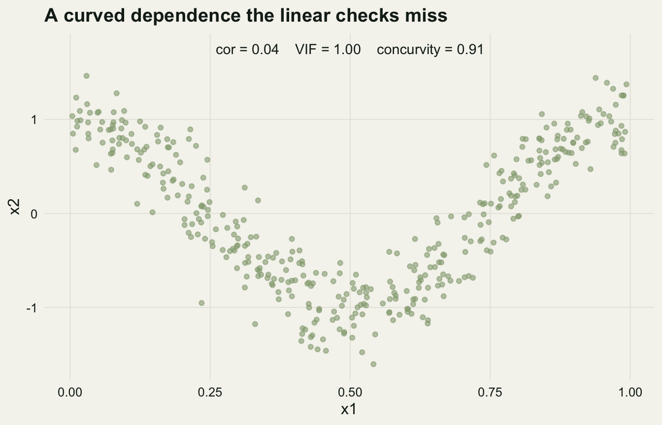
We take a covariate `x1` on the unit interval and set `x2` to a cosine of `x1` plus a little noise. Over this range the cosine is symmetric enough that `x1` and `x2` are almost uncorrelated. The response depends only on `x1`, through a cosine effect; `x2` has no direct role at all.
```{r}
#| label: setup
#| message: false
#| warning: false
#| code-fold: true
#| code-summary: "Setup: packages, colours and plot theme"
library(mgcv)
library(ggplot2)
theme_te <- function() {
  theme_minimal(base_size = 12) +
    theme(
      panel.grid.minor = element_blank(),
      panel.grid.major = element_line(colour = "#e5e4dc", linewidth = 0.3),
      plot.background  = element_rect(fill = "#f5f4ee", colour = NA),
      panel.background = element_rect(fill = "#f5f4ee", colour = NA),
      strip.text = element_text(colour = "#16241d", face = "bold"),
      text      = element_text(colour = "#16241d"),
      axis.text = element_text(colour = "#16241d"),
      plot.title = element_text(face = "bold")
    )
}
col_truth <- "#16241d"; col_naive <- "#c0622d"
col_corr  <- "#275139"; col_sage <- "#93a87f"
```
```{r}
#| label: simulate
#| echo: true
set.seed(4208)
n <- 400
x1 <- runif(n)
x2 <- cos(2 * pi * x1) + rnorm(n, 0, 0.25)   # a curved function of x1
g  <- function(z) 1.6 * cos(2 * pi * z)      # true effect of x1 only
y  <- g(x1) + rnorm(n, 0, 0.6)               # x2 has no direct effect
d  <- data.frame(x1 = x1, x2 = x2, y = y)

p8_cor <- cor(x1, x2)
p8_vif <- 1 / (1 - summary(lm(x2 ~ x1))$r.squared)   # linear VIF of x2 given x1
```
The linear diagnostics report nothing wrong. The correlation between `x1` and `x2` is `r sprintf("%.2f", p8_cor)`, and the variance inflation factor of `x2` given `x1` is `r sprintf("%.2f", p8_vif)`, the value you would see for two unrelated predictors. A collinearity screen based on correlation or variance inflation, the standard advice for linear models, gives this pair a clean pass.
```{r}
#| label: fig-scatter
#| echo: false
#| fig-width: 7
#| fig-height: 4.5
#| fig-cap: "The two covariates trace a cosine, a tight curved relationship, yet their linear correlation is near zero. A variance inflation factor sees independence; concurvity sees the dependence."
#| fig-alt: "Scatter plot of x2 against x1 forming a clear cosine wave, annotated with correlation near zero, variance inflation factor of one, and concurvity of about nine tenths."
p8_cw <- concurvity(gam(y ~ s(x1) + s(x2), data = d, method = "REML"),
full = TRUE)["worst", "s(x2)"]
ggplot(d, aes(x1, x2)) +
geom_point(colour = col_sage, alpha = 0.6, size = 1.4) +
annotate("text", x = 0.5, y = 1.75,
label = sprintf("cor = %.2f VIF = %.2f concurvity = %.2f", p8_cor, p8_vif, p8_cw),
colour = col_truth, size = 3.8) +
labs(x = "x1", y = "x2", title = "A curved dependence the linear checks miss") +
theme_te()
```
## The fitted smooth under both models
Now fit the additive model two ways: the naive model with both smooths, and the correct model with `x1` alone. Because `x2` carries the same cosine information as the true effect, the naive model has two routes to the signal and splits it between them.
```{r}
#| label: fit-both
#| echo: true
naive <- gam(y ~ s(x1) + s(x2), data = d, method = "REML")
corr  <- gam(y ~ s(x1),          data = d, method = "REML")
sm <- summary(naive)
p8_edf_x1 <- sm$edf[1]; p8_p_x1 <- sm$s.pv[1]
p8_edf_x2 <- sm$edf[2]; p8_p_x2 <- sm$s.pv[2]

## compare each fit to the true effect on a grid
xg <- seq(0.02, 0.98, length = 100)
gt <- g(xg) - mean(g(x1))                      # centred truth
pn <- predict(naive, data.frame(x1 = xg, x2 = 0), type = "terms")[, "s(x1)"]
pc <- predict(corr,  data.frame(x1 = xg),         type = "terms")[, "s(x1)"]
p8_rmse_naive <- sqrt(mean((pn - gt)^2))
p8_rmse_corr  <- sqrt(mean((pc - gt)^2))
```
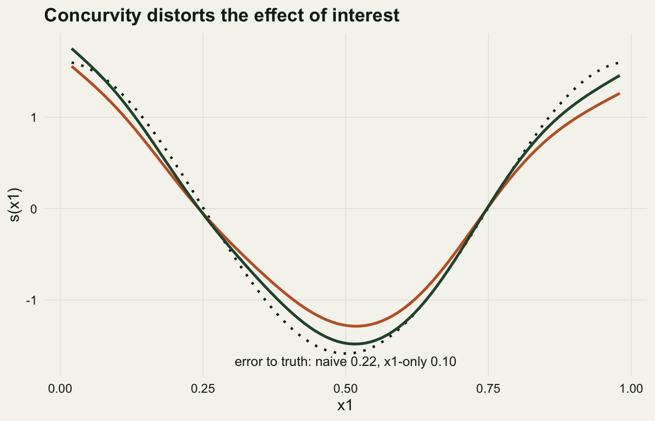
The `x1` smooth is the term we care about. Measured against the true effect, the `x1` smooth from the naive model sits `r sprintf("%.3f", p8_rmse_naive)` away and the smooth from the `x1`-only model `r sprintf("%.3f", p8_rmse_corr)`. The distance in a single fit is not the diagnostic; the concurvity of the design is, and the section below measures it. Meanwhile the noise variable `x2` picks up a smooth of `r sprintf("%.1f", p8_edf_x2)` effective degrees of freedom with a p-value of `r sprintf("%.2f", p8_p_x2)`: not quite flagged here.
```{r}
#| label: fig-terms
#| echo: false
#| fig-width: 7
#| fig-height: 4.5
#| fig-cap: "The estimated effect of x1 from the naive model with s(x2) (orange), from the x1-only model (green), and the true effect (dotted). The orange curve departs from the other two, even though x2 has no real effect."
#| fig-alt: "Three curves for the effect of x1 against x1: a dotted true cosine, a green x1-only estimate lying close to it, and an orange naive estimate that departs from both, especially near the peaks and troughs."
gr <- data.frame(x1 = xg, naive = pn, corr = pc, tru = gt)
ggplot(gr, aes(x1)) +
geom_line(aes(y = tru), colour = col_truth, linetype = "dotted", linewidth = 0.9) +
geom_line(aes(y = naive), colour = col_naive, linewidth = 1) +
geom_line(aes(y = corr), colour = col_corr, linewidth = 1) +
annotate("text", x = 0.5, y = min(gt) * 1.05,
label = sprintf("error to truth: naive %.2f, x1-only %.2f",
p8_rmse_naive, p8_rmse_corr),
colour = col_truth, size = 3.6) +
labs(x = "x1", y = "s(x1)",
title = "The x1 smooth under both models") +
theme_te()
```
## Reproducing the concurvity measure
The `concurvity` function in `mgcv` quantifies the overlap. For each smooth it reports how much of that term can be reproduced by the others, on a scale from zero to one. We can reproduce its estimate directly: build the model matrix, project the `x2` block onto the space spanned by the intercept and the `x1` block, and take the fraction of the `x2` block that projection explains.
```{r}
#| label: concurvity
#| echo: true
cfull <- concurvity(naive, full = TRUE)
p8_cw <- cfull["worst", "s(x2)"]; p8_ce <- cfull["estimate", "s(x2)"]

X <- predict(naive, type = "lpmatrix")
idx <- lapply(naive$smooth, function(s) s$first.para:s$last.para)
X2 <- X[, idx[[2]], drop = FALSE]
Xother <- cbind(1, X[, idx[[1]], drop = FALSE])
proj <- Xother %*% solve(crossprod(Xother), t(Xother))
p8_hand <- sum(diag(t(X2) %*% proj %*% X2)) / sum(diag(crossprod(X2)))
```
The hand projection gives `r sprintf("%.3f", p8_hand)`, matching mgcv's estimate of `r sprintf("%.3f", p8_ce)` exactly. Its worst-case measure is higher still, `r sprintf("%.2f", p8_cw)`. That measure maximises over the whole `x2` term space: it is the share explained for the function in that space which the intercept and the `x1` block reproduce best, not the overlap of the fitted `x2` smooth. A concurvity that high is a warning that the split between the two terms is close to arbitrary.
## How often does the noise slip through?
A single fit understates the instability. We resample the data and refit, tracking the magnitude the model assigns to each smooth, and we run a separate simulation counting how often the noise variable is declared significant when it has no effect.
```{r}
#| label: simulations
#| echo: true
set.seed(7)
Bb <- 300; s2mag <- numeric(Bb)
for (b in 1:Bb) {
  ii <- sample(n, replace = TRUE); db <- d[ii, ]
  mb <- gam(y ~ s(x1) + s(x2), data = db, method = "REML")
  s2mag[b] <- sd(predict(mb, type = "terms")[, "s(x2)"])
}
p8_boot_med <- median(s2mag)
p8_boot_lo  <- quantile(s2mag, 0.05); p8_boot_hi <- quantile(s2mag, 0.95)

set.seed(2020)
Bm <- 500; sig <- 0
for (b in 1:Bm) {
  a1 <- runif(n); a2 <- cos(2 * pi * a1) + rnorm(n, 0, 0.25)
  yy <- g(a1) + rnorm(n, 0, 0.6)
  if (summary(gam(yy ~ s(a1) + s(a2), method = "REML"))$s.pv[2] < 0.05) sig <- sig + 1
}
p8_type1 <- sig / Bm
```
Across resamples the size the model gives to the `x2` smooth has a middle 90 per cent running from `r sprintf("%.2f", p8_boot_lo)` to `r sprintf("%.2f", p8_boot_hi)`, with a median of `r sprintf("%.2f", p8_boot_med)`. The partition is unstable: some samples hand the noise variable a real share of the signal. And in the null simulation the noise variable is flagged at the 0.05 level `r sprintf("%.0f%%", 100 * p8_type1)` of the time. This is the same anti-conservative failure Ramsay and colleagues described for concurvity in air pollution time series: the standard errors are too small, so the tests reject too often.
## Living with concurvity
Concurvity, like collinearity, is a property of the design, not a flaw in the estimator. No cleverer fitting method separates the effects of `x1` and `x2` when the data cannot: if one smooth is a curved copy of another, their individual contributions are not identifiable, and the worst-case concurvity measures how bad that can get. The remedies are the same as for collinearity in spirit. If `x2` is a proxy or a nuisance, drop it. If both are of scientific interest and genuinely interact, model that interaction directly rather than as two competing marginal smooths. If neither is possible, report the concurvity and treat the separate effects as what they are, weakly identified.
The practical habit is to run `concurvity` alongside `k.check` whenever a model has several smooths, and to remember that a clean correlation matrix is not evidence of independence. The dependence that hurts an additive model is curved, and only a measure built for curves will see it.
## References
Ramsay TO, Burnett RT, Krewski D 2003. Epidemiology 14(1):18-23 (10.1097/00001648-200301000-00009).
Buja A, Hastie T, Tibshirani R 1989. The Annals of Statistics 17(2):453-510 (10.1214/aos/1176347115).
Dormann CF, Elith J, Bacher S, Buchmann C, Carl G, et al. 2013. Ecography 36(1):27-46 (10.1111/j.1600-0587.2012.07348.x).
Wood SN 2017. Generalized Additive Models: An Introduction with R, 2nd edn. CRC Press. ISBN 978-1-4987-2833-1.
Zuur AF, Ieno EN, Walker NJ, Saveliev AA, Smith GM 2009. Mixed Effects Models and Extensions in Ecology with R. Springer. ISBN 978-0-387-87457-9.
## Related tutorials
- [Penalised regression splines from scratch](../penalised-regression-splines/)
- [Checking a generalised additive model](../checking-a-gam/)
- [Collinearity and the variance inflation factor](../collinearity-and-vif/)
- [Spatial+ and the attenuated slope](../spatial-plus-and-the-attenuated-slope/)