---
title: "Modeling nonlinear species responses with GAMs"
description: "A count GLM forces a single direction of response. When a species peaks at an intermediate optimum, a generalized additive model lets the data choose the shape."
date: "2026-06-22 12:00"
categories: [R, regression, GAMs, mgcv]
image: thumbnail.png
image-alt: "Three fitted curves over count data: a flat line, a symmetric parabola, and a skewed smooth that tracks the data."
---
The [previous post on count GLMs](../glm-count-data-abundance/) modeled abundance with a log link and a linear predictor. On the count scale that gives a monotonic curve: abundance climbs (or falls) without turning around. For many species that is the wrong shape. A species tends to be most common somewhere near the middle of its tolerance and rarer at both ends of a gradient, the picture behind gradient analysis (ter Braak and Prentice 1988). A model that can only go one direction cannot represent a peak.
There is a familiar parametric patch: add a squared term. On the log scale a quadratic bends, so `exp` of it gives a hump. That recovers the symmetric Gaussian response, but it forces the rise and the fall to mirror each other. Real responses are often lopsided: a slow approach to the optimum and a sharp drop past it, or the reverse.
Generalized additive models (Hastie and Tibshirani 1986) replace the fixed functional form with a penalized smooth. The smooth can be a line, a parabola, or something skewed, and the penalty decides how much it is allowed to bend based on the data. Yee and Mitchell (1991) brought them into plant ecology for exactly this question: is a response curve symmetric and bell shaped, or not? This post fits one species three ways, then uses a single smooth on four species with different true shapes.
## A species with a skewed optimum
The gradient is a single environmental axis (read it as a moisture or productivity index). The species has its optimum at the upper-middle of the range, rises gently from the dry end, and drops steeply once past the peak. Counts are negative binomial, so they carry the overdispersion that the count GLM post dealt with.
```{r}
#| label: simulate
#| warning: false
#| message: false
library(mgcv)
library(MASS)
library(ggplot2)

set.seed(91)
n    <- 200
grad <- runif(n, 0, 10)                       # environmental gradient
opt  <- 6.5; wL <- 3.0; wR <- 1.2; peak <- 26 # gentle rise, steep fall
w    <- ifelse(grad < opt, wL, wR)
mu   <- peak * exp(-0.5 * ((grad - opt) / w)^2)
count <- rnbinom(n, mu = mu, size = 2.0)       # overdispersed counts
d <- data.frame(grad, count)

c(n = n, max = max(count), mean = round(mean(count), 1), zeros = sum(count == 0))
```
About two hundred plots, counts from zero into the low fifties, with a fair share of zeros at the gradient ends.
## Three models for one response
The linear negative binomial GLM is the monotonic baseline. The quadratic GLM adds a squared term, the symmetric hump. The GAM puts a single smooth on the gradient and lets it find its own shape.
```{r}
#| label: fit
#| warning: false
#| message: false
m_lin <- glm.nb(count ~ grad, data = d)
m_qua <- glm.nb(count ~ grad + I(grad^2), data = d)
m_gam <- gam(count ~ s(grad), family = nb(), method = "REML", data = d)

AIC(m_lin, m_qua, m_gam)
```
The linear model is far behind. Its slope is small and barely separable from zero, because averaged over the whole gradient a humped response has almost no net direction: the rise and the fall cancel. The quadratic recovers a clear peak and drops the AIC by more than a hundred. The GAM improves on the quadratic by a handful of AIC, which is modest but real, and the reason is shape.
```{r}
#| label: smooth-summary
#| warning: false
#| message: false
summary(m_gam)$s.table
```
The smooth uses around five effective degrees of freedom and is strongly significant. The model accounts for roughly forty-four percent of the deviance. Five degrees of freedom is more bend than a parabola has, which is the signature of asymmetry: the quadratic spends its single curvature on a symmetric arc, while the smooth keeps some left over to flatten one shoulder and steepen the other.
```{r}
#| label: fig-three
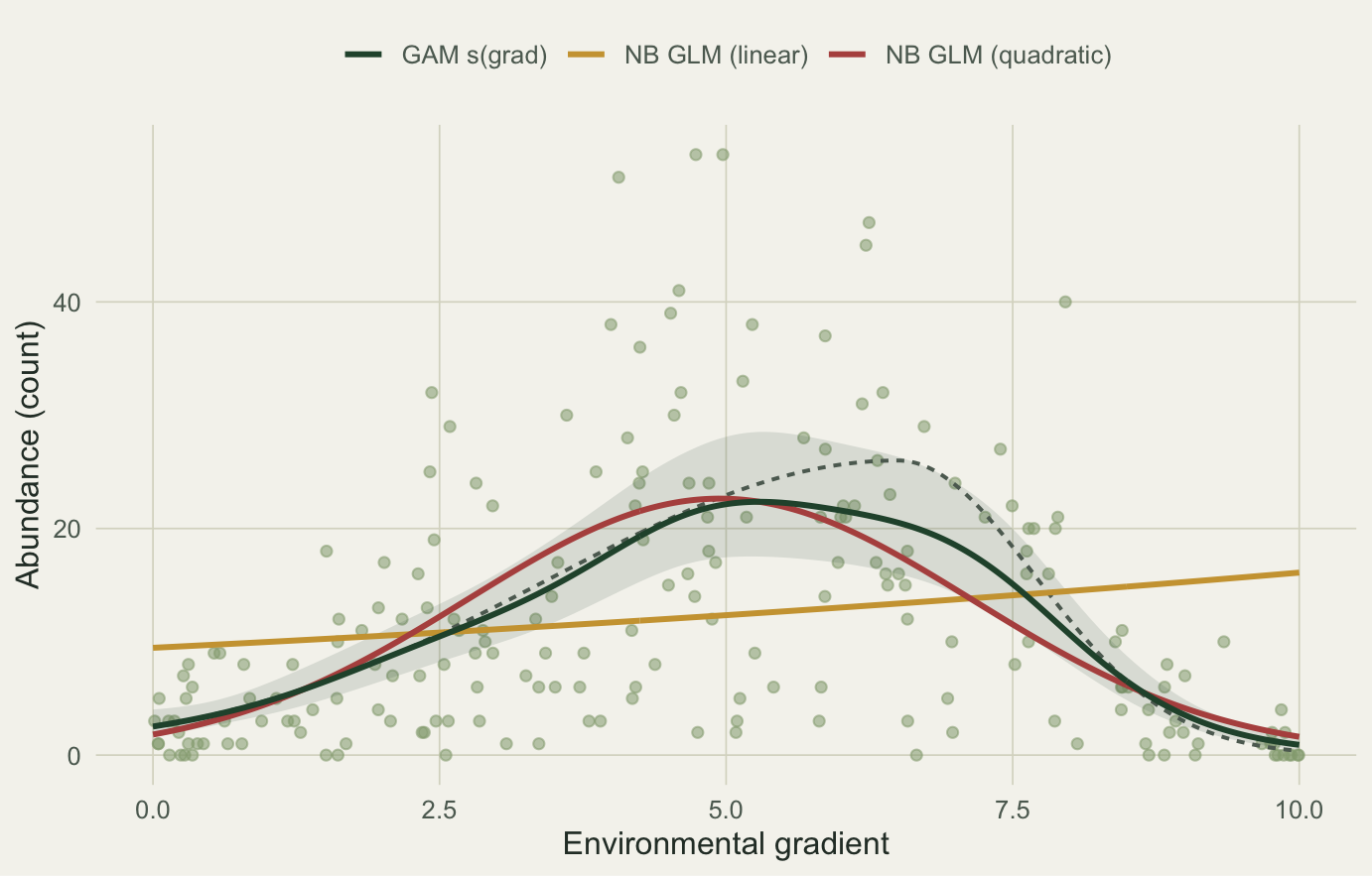
#| fig-cap: "One species, three models. The dashed grey line is the true skewed response. The linear fit stays flat, the quadratic is a symmetric arc, and the smooth follows the lopsided shape."
#| fig-width: 7.2
#| fig-height: 4.6
#| warning: false
#| message: false
#| echo: false
pal <- list(paper="#f5f4ee", ink="#16241d", body="#2c3a31", forest="#275139",
line="#dad9ca", sage="#93a87f", gold="#cda23f", terra="#b5534e",
faint="#5d6b61")
theme_te <- function(base=12){
theme_minimal(base_size=base) +
theme(panel.grid.minor=element_blank(),
panel.grid.major=element_line(color=pal$line, linewidth=.3),
plot.background=element_rect(fill=pal$paper, color=NA),
panel.background=element_rect(fill=pal$paper, color=NA),
axis.title=element_text(color=pal$body), axis.text=element_text(color=pal$faint),
plot.title=element_text(color=pal$ink, face="bold"),
plot.subtitle=element_text(color=pal$faint),
strip.text=element_text(color=pal$ink, face="bold"),
legend.text=element_text(color=pal$faint), legend.position="top")
}
xs <- data.frame(grad = seq(0, 10, length.out = 300))
xs$true <- peak * exp(-0.5 * ((xs$grad - opt) / ifelse(xs$grad < opt, wL, wR))^2)
xs$lin <- predict(m_lin, xs, type = "response")
xs$qua <- predict(m_qua, xs, type = "response")
pg <- predict(m_gam, xs, type = "link", se.fit = TRUE); ig <- m_gam$family$linkinv
xs$gam <- ig(pg$fit); xs$lo <- ig(pg$fit - 1.96*pg$se.fit); xs$hi <- ig(pg$fit + 1.96*pg$se.fit)
cols <- c("NB GLM (linear)"=pal$gold, "NB GLM (quadratic)"=pal$terra, "GAM s(grad)"=pal$forest)
ggplot() +
geom_point(data = d, aes(grad, count), color = pal$sage, alpha = .55, size = 1.6) +
geom_ribbon(data = xs, aes(grad, ymin = lo, ymax = hi), fill = pal$forest, alpha = .13) +
geom_line(data = xs, aes(grad, true), color = pal$faint, linetype = "22", linewidth = .7) +
geom_line(data = xs, aes(grad, lin, color = "NB GLM (linear)"), linewidth = 1.05) +
geom_line(data = xs, aes(grad, qua, color = "NB GLM (quadratic)"), linewidth = 1.05) +
geom_line(data = xs, aes(grad, gam, color = "GAM s(grad)"), linewidth = 1.05) +
scale_color_manual(values = cols, name = NULL) +
labs(x = "Environmental gradient", y = "Abundance (count)") +
theme_te()
```
The shaded band is the smooth's ninety-five percent interval. Notice it widens where the data thin out near the peak: the exact position of the optimum is genuinely uncertain with this much noise, and the GAM says so rather than pretending to a precise turning point. Both humped models place the apparent optimum a little below the true value, pulled left by the steep right tail and the scatter. That is a property of the data, not a failure of either model.
## Is the basis big enough?
A smooth is built from a fixed number of basis functions; `k` sets the ceiling on flexibility. If the true response needs more wiggliness than `k` allows, the fit is biased. `gam.check` (here just its numeric part) tests whether the residuals still hold pattern that a larger basis could catch.
```{r}
#| label: kcheck
#| warning: false
#| message: false
k.check(m_gam)
```
The effective degrees of freedom sit well under the basis size, and the test is not significant, so the default basis is adequate. If `k'` and `edf` were close and the p value small, the move is to refit with a larger `k`.
## One smooth, four shapes
The same `s(grad)` term handles whatever the data show. Here are four species: one rising, one falling, one with a symmetric optimum, and the skewed one from above. Each gets its own GAM, with nothing changed but the data.
```{r}
#| label: fig-panel
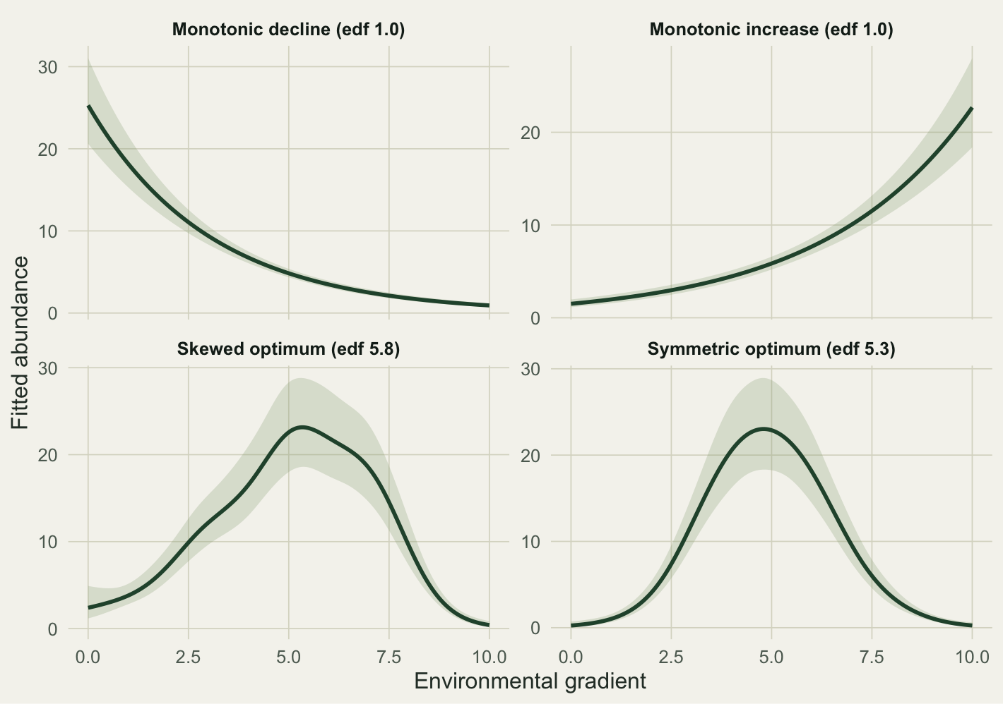
#| fig-cap: "A single smooth term fit to four species. The two monotonic species collapse to one effective degree of freedom; the two humped species use around five. The penalty reads the shape off the data."
#| fig-width: 7.4
#| fig-height: 5.2
#| warning: false
#| message: false
set.seed(112)
g2 <- runif(220, 0, 10)
make_sp <- function(grad, shape) {
  mu <- switch(shape,
    increasing = exp(0.2 + 0.30 * grad),
    decreasing = exp(3.2 - 0.34 * grad),
    symmetric  = 24 * exp(-0.5 * ((grad - 5) / 1.6)^2),
    skewed     = 24 * exp(-0.5 * ((grad - 6.5) / ifelse(grad < 6.5, 3.0, 1.2))^2))
  rnbinom(length(grad), mu = mu, size = 2)
}
shapes <- c("increasing", "decreasing", "symmetric", "skewed")
labs2  <- c(increasing = "Monotonic increase", decreasing = "Monotonic decline",
            symmetric = "Symmetric optimum", skewed = "Skewed optimum")

panel <- do.call(rbind, lapply(shapes, function(s) {
  cnt <- make_sp(g2, s)
  mod <- gam(cnt ~ s(grad), family = nb(), method = "REML",
             data = data.frame(grad = g2, cnt = cnt))
  ed  <- summary(mod)$s.table[1, "edf"]
  xs2 <- data.frame(grad = seq(0, 10, length.out = 200))
  pr  <- predict(mod, xs2, type = "link", se.fit = TRUE); iv <- mod$family$linkinv
  data.frame(grad = xs2$grad, fit = iv(pr$fit),
             lo = iv(pr$fit - 1.96*pr$se.fit), hi = iv(pr$fit + 1.96*pr$se.fit),
             species = sprintf("%s (edf %.1f)", labs2[[s]], ed))
}))

ggplot(panel, aes(grad, fit)) +
  geom_ribbon(aes(ymin = lo, ymax = hi), fill = pal$sage, alpha = .25) +
  geom_line(color = pal$forest, linewidth = 1) +
  facet_wrap(~species, scales = "free_y") +
  labs(x = "Environmental gradient", y = "Fitted abundance") +
  theme_te() + theme(legend.position = "none")
```
The two monotonic species come back at one effective degree of freedom. The penalty has looked at the data and decided a straight line on the link scale is all they support, so the smooth does not invent curvature that is not there. The two humped species use around five. This is the practical read on `edf`: near one means a line suffices, well above one means the response bends. It is not a polynomial degree, and it is specific to this sample; a noisier draw of the same species can land on a different number.
## When to reach for which
The smooth earns its place when you do not want to commit to a shape in advance, when the response might be asymmetric, or when you are exploring what the gradient does before settling on a model. The cost is interpretability: a GLM hands you `exp(coefficient)` as a multiplicative effect, while a GAM hands you a curve and a figure. If your question is about a specific parametric form, for example whether a Gaussian (symmetric) response holds, fit that form and test it; Yee and Mitchell (1991) framed the symmetry question this way. If your question is what shape the data prefer, let the smooth answer.
A few working notes. Fit with `method = "REML"`; it penalizes more honestly than the older GCV default and is less prone to undersmoothing. Check `k` whenever a smooth pushes toward its ceiling. And do not read a fitted curve past the range of the data: a smooth has nothing to anchor it in the extrapolated region, and the interval there is wishful.
## References
Hastie, T. and Tibshirani, R. (1986). Generalized additive models. *Statistical Science* 1(3): 297-310. https://doi.org/10.1214/ss/1177013604
Yee, T. W. and Mitchell, N. D. (1991). Generalized additive models in plant ecology. *Journal of Vegetation Science* 2(5): 587-602. https://doi.org/10.2307/3236170
ter Braak, C. J. F. and Prentice, I. C. (1988). A theory of gradient analysis. *Advances in Ecological Research* 18: 271-317. https://doi.org/10.1016/S0065-2504(08)60183-X
Wood, S. N. (2017). *Generalized Additive Models: An Introduction with R*, 2nd edition. Chapman and Hall/CRC. https://doi.org/10.1201/9781315370279