Heteroscedasticity and limiting factors

When an ecological variable sets an upper bound, the mean slope is about half of it. Upper quantiles recover the limiting relationship in base R.

Many ecological scatter plots are wedge-shaped: points spread widely beneath an upper edge that rises with the predictor. The standard reading is the principle of limiting factors. At any site the response is held down by whichever resource is scarcest; the measured variable sets a ceiling on what is possible, and other unmeasured factors push most sites below it. The ecological information then lives in the upper edge, not the middle. A mean regression, which chases the centre, systematically understates the effect of the measured factor when that factor is not the active constraint (Thomson and colleagues 1996; Cade and Noon 2003).

This post shows the pattern with a simple generating model, measures how badly least squares understates the ceiling, and uses upper quantiles to recover it. It also states the honest limit: the same wedge is produced by ordinary changing variance, and the data alone cannot tell the two apart.

A ceiling with scatter beneath it

We build a ceiling that rises with the gradient and let each point fall a random fraction of the way below it. With the fraction drawn uniformly, the tau-quantile of the response given x is exactly tau times the ceiling, so the quantile slope should equal tau times the ceiling slope.

set.seed(4203)
n  <- 300
x  <- runif(n, 1, 20)          # resource gradient (for example patch area)
u  <- runif(n)                 # everything else that can limit a site
b0 <- 2; b1 <- 1.5             # ceiling = b0 + b1 * x
y  <- (b0 + b1 * x) * u        # each site sits somewhere below its ceiling

ols <- lm(y ~ x)
coef(ols)[2]

        x 
0.7313574 

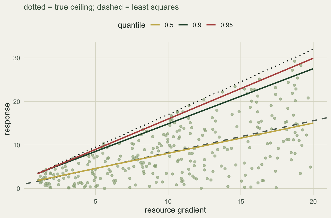
The least-squares slope is 0.731, against a true ceiling slope of 1.5. The ratio is 0.488, close to one half, exactly what you expect: averaging over a uniform fraction of the ceiling gives half the ceiling slope. Read as an effect size, the mean regression halves the strength of the relationship.

Upper quantiles recover the ceiling

Fitting quantile slopes across a range of tau shows the slope climbing toward the ceiling slope as tau increases.

taus <- c(0.5, 0.75, 0.9, 0.95, 0.99)
qs   <- sapply(taus, function(t) qslope(x, y, t))
names(qs) <- taus
round(qs, 3)

  0.5  0.75   0.9  0.95  0.99 
0.696 1.063 1.268 1.396 1.450 

The slopes are 0.696 at the median, rising to 1.268 at the ninetieth and 1.45 at the ninety-ninth percentile, approaching the ceiling slope of 1.5. The theoretical values, tau times the ceiling slope, are 0.75, 1.35 and 1.485. The upper quantiles estimate the limiting relationship that the mean misses.

Figure 1: A wedge under a rising ceiling. Upper quantiles track the bound; least squares (dashed) sits far below it.

The fanning is the signature, and a test for it

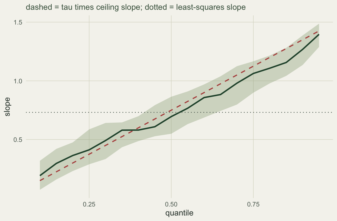
Under constant variance every quantile slope is the same and the fits are parallel. A slope that climbs with tau is the fingerprint of a changing spread, here driven by the limiting-factor structure. A case-resampling bootstrap gives a confidence interval for the difference between an upper and a central slope, which tests whether the fan is real.

set.seed(101)
B  <- 1200
bs <- replicate(B, {
  i <- sample(n, n, TRUE)
  c(qslope(x[i], y[i], 0.5), qslope(x[i], y[i], 0.9))
})
diff_ci <- quantile(bs[2, ] - bs[1, ], c(.025, .975))
round(diff_ci, 3)

 2.5% 97.5% 
0.398 0.737 

The median slope has interval [0.55, 0.869] and the ninetieth [1.139, 1.386]. Their difference is [0.398, 0.737], well clear of zero, so the slopes genuinely differ across the distribution. The whole quantile process makes the point visually.

Figure 2: Slope as a function of tau, with a bootstrap band. It rises toward the ceiling slope; the mean slope (dotted) sits near the middle.

The honest limit

The upper quantile is an honest description of the upper edge of the data. Reading it as a limiting factor is an ecological interpretation, not a statistical result. A wedge like this can equally be produced by a mean relationship with variance that happens to grow with x, with no ceiling and no limiting mechanism at all. The quantile fit is the same in both cases; the fanning slope is the same; the bootstrap interval is the same. Nothing in the data distinguishes a real constraint from ordinary heteroscedasticity. That separation has to come from the ecology: an argument about which resource is scarce, an experiment that manipulates it, or independent knowledge of the mechanism. Quantile regression tells you where the edge is and how steep it is; it does not tell you why the points sit below it (Cade, Noon and Flather 2005).

References

Cade and Noon 2003 Frontiers in Ecology and the Environment 1(8):412-420 (10.1890/1540-9295(2003)001[0412:AGITQR]2.0.CO;2)

Cade, Terrell and Schroeder 1999 Ecology 80(1):311-323 (10.1890/0012-9658(1999)080[0311:EEOLFW]2.0.CO;2)

Thomson, Weiblen, Thomson, Alfaro and Legendre 1996 Ecology 77(6):1698-1715 (10.2307/2265776)

Scharf, Juanes and Sutherland 1998 Ecology 79(2):448-460 (10.1890/0012-9658(1998)079[0448:IERFTE]2.0.CO;2)

Cade, Noon and Flather 2005 Ecology 86(3):786-800 (10.1890/04-0785)

Related tutorials

• Quantile regression in ecology: beyond the mean
• Distributional regression with location and scale
• Checking a quantile regression
• Species response curves with GAMs