Distributional regression with location and scale

Model the spread, not just the mean. A base-R location-scale fit, why naive prediction intervals miscalibrate, and how it connects to quantile regression.

Quantile regression describes the shape of a conditional distribution without naming it. A complementary route is to name a distribution and let more than its mean depend on the predictor. The simplest version is a location-scale model: the response is Gaussian, its mean is a function of the covariate, and so is its standard deviation. When the spread of an ecological response changes across a gradient, the mean slope is often beside the point and the variance slope is the finding. This post fits such a model in base R with optim, shows why a mean-only model gives the wrong prediction intervals, and connects the parametric quantiles it implies to the distribution-free ones from quantile regression.

Mean and spread both depend on the gradient

set.seed(4204)
n  <- 400
x  <- runif(n, 0, 10)
a0 <- 1; a1 <- 0.8              # mean:  a0 + a1 * x
c0 <- log(0.8); c1 <- 0.12     # log standard deviation: c0 + c1 * x
y  <- rnorm(n, a0 + a1 * x, exp(c0 + c1 * x))

coef(lm(y ~ x))[2]             # the mean slope, from ordinary least squares

        x 
0.7946731 

The mean slope is easy: least squares estimates it well. The mean-only model then assumes a single standard deviation for the whole gradient, which is wrong here by construction. To recover the spread, we write the negative log-likelihood with the mean as one linear predictor and the log standard deviation as another, and minimise it:

nll <- function(p, X, Z, y) {
  k <- ncol(X); b <- p[1:k]; g <- p[(k + 1):(k + ncol(Z))]
  s <- exp(as.vector(Z %*% g))
  -sum(dnorm(y, as.vector(X %*% b), s, log = TRUE))
}
X <- cbind(1, x); Z <- cbind(1, x)
ols <- lm(y ~ x)
fit <- optim(c(unname(coef(ols)), log(sd(resid(ols))), 0),
             nll, X = X, Z = Z, y = y, method = "BFGS", hessian = TRUE)
bML <- fit$par[1:2]; gML <- fit$par[3:4]
se  <- sqrt(diag(solve(fit$hessian)))
c(mean_slope = bML[2], logsd_slope = gML[2])

 mean_slope logsd_slope 
  0.8022058   0.1318442 

The two models agree on the mean slope (0.795 from least squares, 0.802 from the location-scale fit): that is not where they differ. The location-scale fit adds the log standard deviation slope, 0.132 with standard error 0.011, against a true value of 0.12. A likelihood-ratio test of this one extra parameter is decisive: the statistic is 123.61 on one degree of freedom (p = 1.03^{-28}), and the varying-spread model improves the AIC by 121.6. The spread is the signal, and a mean-only model is blind to it.

Why the naive prediction interval is wrong

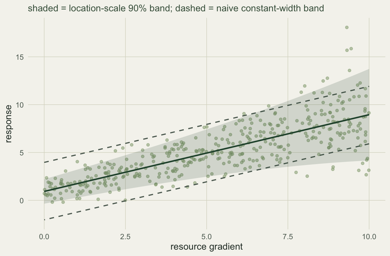
A mean-only model builds a prediction interval of constant width from the residual standard deviation. Where the true spread is small that band is too wide; where it is large it is too narrow. We can measure this on a fresh, large sample by checking how often the response falls inside a nominal ninety per cent band.

set.seed(55)
xt <- runif(20000, 0, 10)
yt <- rnorm(20000, a0 + a1 * xt, exp(c0 + c1 * xt))
z90 <- qnorm(0.95)
covN <- abs(yt - (coef(ols)[1] + coef(ols)[2] * xt)) <= z90 * sdm
covL <- abs(yt - (bML[1] + bML[2] * xt)) <= z90 * exp(gML[1] + gML[2] * xt)
terc <- cut(xt, quantile(xt, c(0, 1/3, 2/3, 1)), include.lowest = TRUE,
            labels = c("low", "mid", "high"))
rbind(naive = tapply(covN, terc, mean), locscale = tapply(covL, terc, mean))

               low       mid      high
naive    0.9961002 0.9582958 0.8362082
locscale 0.8942553 0.9086409 0.9271036

Averaged over the whole gradient the naive band looks passable (0.93 against a target of 0.90). Split by thirds it falls apart: it covers 0.996 of points in the low-spread region and only 0.836 in the high-spread region. The location-scale band, whose width tracks the fitted standard deviation, stays near the target everywhere: 0.894 low, 0.927 high, 0.91 overall. Averaging hides the miscalibration; modelling the spread removes it.

Figure 1: The location-scale band (shaded) widens with the spread; the naive constant-width band (dashed) is too wide at low x and too narrow at high x.

The bridge to quantile regression

A location-scale model implies quantiles directly: the tau-quantile is the fitted mean plus the standard normal quantile times the fitted standard deviation. Quantile regression estimates the same curves without assuming a distribution. When the Gaussian assumption holds, the two agree closely.

xg <- seq(0, 10, length.out = 60)
agree <- sapply(c(0.1, 0.9), function(tt) {
  para <- (bML[1] + bML[2] * xg) + qnorm(tt) * exp(gML[1] + gML[2] * xg)
  qc   <- qrfit(x, y, tt)
  cor(para, qc[1] + qc[2] * xg)
})
round(agree, 4)

[1] 0.9964 0.9991

The fitted parametric and distribution-free quantile curves line up almost exactly, with correlations 0.9964 at the tenth percentile and 0.9991 at the ninetieth. Under a correct family the parametric route is more efficient: it borrows strength across the whole distribution to pin down each quantile.

The honest limit: the family is a choice

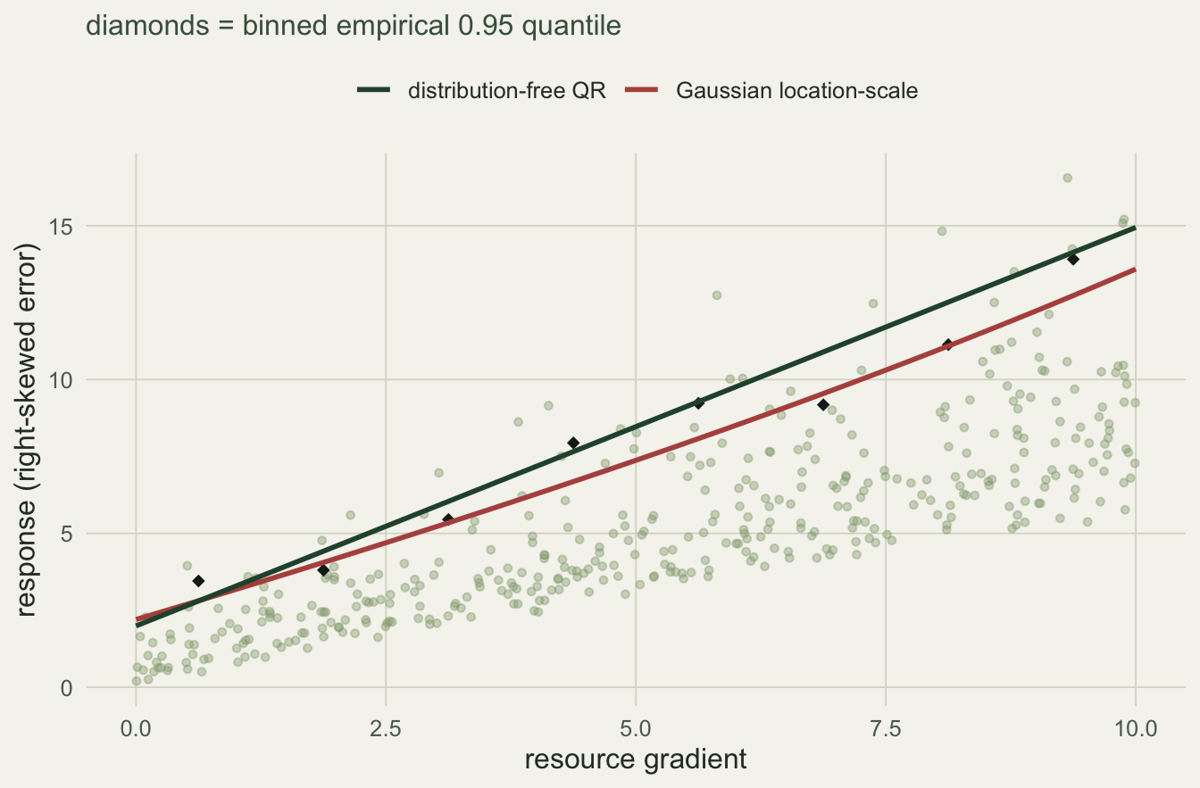
Efficiency comes at the price of an assumption. The location-scale model treats the errors as symmetric and Gaussian, and it is the tails that pay when that is wrong. If the errors are skewed, the true ninety-fifth percentile is not the fitted mean plus 1.645 standard deviations, and the parametric quantile drifts off exactly where you most want it. Quantile regression, which makes no such assumption, holds up. We test both on right-skewed errors, checking how often the response falls below each fitted ninety-fifth-percentile line on a large sample.

set.seed(4214)
e0 <- (rgamma(n, 2, 1) - 2) / sqrt(2)          # standardised right-skewed error
ys <- (a0 + a1 * x) + exp(c0 + c1 * x) * e0
fs <- optim(c(unname(coef(lm(ys ~ x))), log(sd(resid(lm(ys ~ x)))), 0),
            nll, X = X, Z = Z, y = ys, method = "BFGS")
bS <- fs$par[1:2]; gS <- fs$par[3:4]
qc95 <- qrfit(x, ys, 0.95)
set.seed(77)
xts <- runif(40000, 0, 10)
yts <- (a0 + a1 * xts) + exp(c0 + c1 * xts) * (rgamma(40000, 2, 1) - 2) / sqrt(2)
gaussQ <- (bS[1] + bS[2] * xts) + qnorm(0.95) * exp(gS[1] + gS[2] * xts)
qrQ    <- qc95[1] + qc95[2] * xts
c(gaussian = mean(yts < gaussQ), quantile_reg = mean(yts < qrQ))

    gaussian quantile_reg 
    0.929075     0.959475 

The target coverage is 0.95. The Gaussian location-scale line reaches only 0.929: it sits too low, because a right-skewed upper tail is heavier than the normal one and the model cannot see that. The distribution-free quantile line reaches 0.959, close to the mark. This is the trade. A distributional model is efficient and gives you the whole distribution at once, but only if the family is right, and the family is a choice you make, not something the data hand you. Quantile regression asks for less and, in the tails, delivers more.

Figure 2: On right-skewed errors the Gaussian ninety-fifth-percentile line sits below the binned empirical quantile; the distribution-free fit tracks it.

References

Rigby and Stasinopoulos 2005 Journal of the Royal Statistical Society Series C 54(3):507-554 (10.1111/j.1467-9876.2005.00510.x)

Kneib 2013 Statistical Modelling 13(4):275-303 (10.1177/1471082X13494159)

Koenker and Bassett 1978 Econometrica 46(1):33-50 (10.2307/1913643)

Yu, Lu and Stander 2003 Journal of the Royal Statistical Society Series D 52(3):331-350 (10.1111/1467-9884.00363)

Koenker 2005 Quantile Regression, Cambridge University Press (ISBN 978-0-521-84573-1)

Related tutorials

• Quantile regression in ecology: beyond the mean
• Heteroscedasticity and limiting factors
• Checking a quantile regression
• Standard errors and confidence intervals