Standard errors and confidence intervals in R

What a standard error and a 95% confidence interval mean in R, how they differ from the standard deviation, and how to check interval coverage by simulation.

Almost every ecological result is a number plus an admission that the number could have come out differently. You sampled 30 plots, not every plot; another 30 would have given another mean. The standard error and the confidence interval are the two tools for putting that uncertainty on the page. They are also two of the most misread quantities in the field, so this post builds them from a known population, checks them by simulation, and shows where the textbook formula quietly breaks.

We will use a population we control, so we always know the right answer. Picture per-plot biomass in grams, right-skewed the way biomass usually is, drawn from a gamma distribution with a true mean of 20 and a true standard deviation of 10.

library(ggplot2)

paper <- "#f5f4ee"; ink <- "#16241d"; forest <- "#275139"
gold  <- "#cda23f"; miss_red <- "#b5534e"; faint <- "#5d6b61"; line <- "#dad9ca"

theme_te <- theme_minimal(base_size = 12) +
  theme(panel.grid.minor = element_blank(),
        panel.grid.major = element_line(colour = line, linewidth = 0.3),
        plot.background = element_rect(fill = paper, colour = NA),
        panel.background = element_rect(fill = paper, colour = NA),
        axis.title = element_text(colour = ink),
        axis.text = element_text(colour = faint),
        plot.title = element_text(colour = ink, face = "bold"))

shape <- 4; rate <- 0.2
mu_true <- shape / rate            # 20
sd_true <- sqrt(shape) / rate      # 10

The standard error is not the standard deviation

Take one sample of 30 plots and measure the spread two ways.

set.seed(101)
n <- 30
x <- rgamma(n, shape, rate)

m  <- mean(x)
s  <- sd(x)            # standard deviation: spread of the data
se <- s / sqrt(n)      # standard error: spread of the mean

round(c(mean = m, sd = s, se = se), 2)

 mean    sd    se 
19.80  8.82  1.61 

The sample mean is 19.8 grams. The standard deviation is 8.82, and the standard error is 1.61, about 5.5 times smaller. That gap is the whole point. The standard deviation answers “how variable are individual plots?” and stays roughly 10 no matter how many plots you measure. The standard error answers “how variable is my estimate of the mean?” and shrinks as the sample grows, because averaging cancels noise. Writing one where you mean the other is the most common error-bar mistake in ecology: standard deviation bars describe the organisms, standard error bars describe your confidence in the average.

The shrinking is exactly \(\text{SE} = \sigma / \sqrt{n}\). Across a grid of sample sizes, the average sample standard deviation sits near the true 10 while the average standard error falls off with the square root of n.

set.seed(202)
ns <- c(5, 10, 20, 40, 80, 160, 320)
grid <- do.call(rbind, lapply(ns, function(nn) {
  reps <- 1500
  sds <- numeric(reps); ses <- numeric(reps)
  for (i in seq_len(reps)) {
    xi <- rgamma(nn, shape, rate)
    sds[i] <- sd(xi); ses[i] <- sd(xi) / sqrt(nn)
  }
  data.frame(n = nn, SD = mean(sds), SE = mean(ses))
}))

long <- rbind(
  data.frame(n = grid$n, value = grid$SD, quantity = "standard deviation"),
  data.frame(n = grid$n, value = grid$SE, quantity = "standard error")
)

ggplot(long, aes(n, value, colour = quantity)) +
  geom_line(linewidth = 1) + geom_point(size = 2) +
  scale_x_log10(breaks = ns) +
  scale_colour_manual(values = c("standard deviation" = forest,
                                 "standard error" = gold)) +
  labs(x = "sample size (n, log scale)", y = "average value (g)",
       colour = NULL,
       title = "Spread of the data versus spread of the estimate") +
  theme_te + theme(legend.position = "top")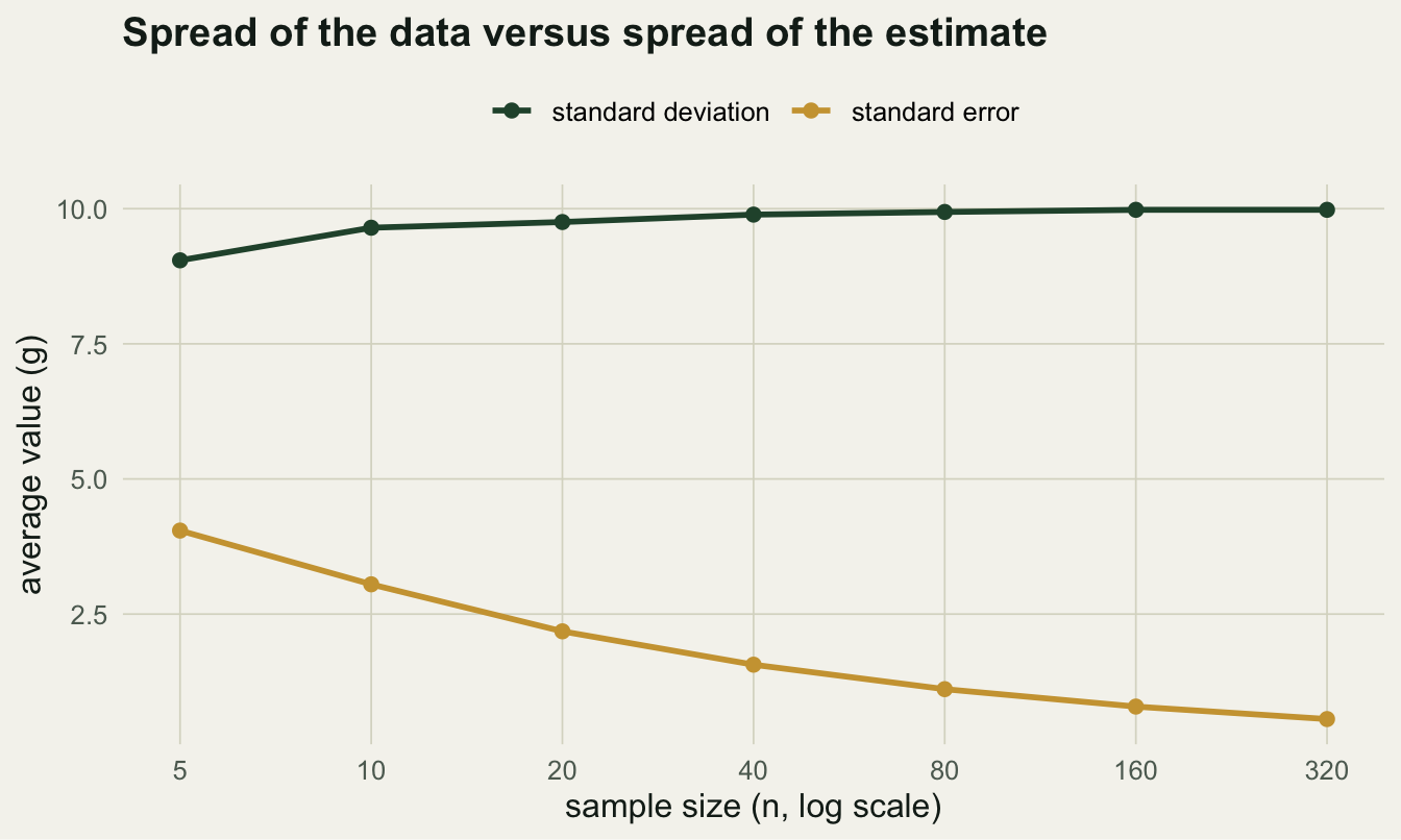

Figure 1: Standard deviation stays near the true value of 10 as sample size grows, while the standard error shrinks with the square root of n. Spread of the data is not spread of the estimate.

Building a 95% confidence interval

A confidence interval turns the standard error into a range. For a mean it is the estimate plus or minus a multiplier from the t distribution times the standard error, where the multiplier accounts for the extra uncertainty of estimating the spread from the same small sample.

tcrit <- qt(0.975, df = n - 1)        # multiplier for 95%, df = n - 1
ci <- m + c(-1, 1) * tcrit * se
round(c(t_multiplier = tcrit, lower = ci[1], upper = ci[2]), 2)

t_multiplier        lower        upper 
        2.05        16.50        23.09 

# the same interval, the easy way
as.numeric(t.test(x)$conf.int)

[1] 16.50317 23.09237

With 29 degrees of freedom the multiplier is 2.05, slightly above the 1.96 you would use if the spread were known exactly. The interval runs from 16.5 to 23.09 grams, and t.test() returns the identical bounds, so the formula and the built-in agree.

Now the interpretation, where care is needed. A 95% confidence interval does not mean there is a 95% probability that the true mean lies inside this particular interval. The true mean is a fixed number; it is either in or out. The 95% is a property of the procedure: if you repeated the whole exercise many times, about 95% of the intervals you build would contain the truth. The confidence is in the method over the long run, not in any single interval. That distinction sounds pedantic until you check it.

Does the procedure deliver? Check coverage by simulation

Because we know the true mean is 20, we can build the interval thousands of times and simply count how often it catches the truth. A well-behaved 95% procedure should land near 95%.

coverage <- function(nn, nsim = 4000, seed) {
  set.seed(seed)
  hit <- 0L
  for (i in seq_len(nsim)) {
    xi <- rgamma(nn, shape, rate)
    lo_hi <- mean(xi) + c(-1, 1) * qt(0.975, nn - 1) * sd(xi) / sqrt(nn)
    if (lo_hi[1] <= mu_true && mu_true <= lo_hi[2]) hit <- hit + 1L
  }
  100 * hit / nsim
}

c(n30 = coverage(30, seed = 303), n5 = coverage(5, seed = 404))

  n30    n5 
94.55 93.50 

At n = 30 the empirical coverage is 94.6%, close to the promised 95%. At n = 5 it slips to 93.5%. The t interval assumes the sampling distribution of the mean is roughly normal, which the central limit theorem delivers for moderate samples even from skewed data, but with only five skewed observations the approximation is not quite there and the interval is a touch too narrow. The lesson is not that the method is broken; it is that “95%” is earned by sample size and shape, and is worth verifying rather than assuming.

The figure below makes the long-run idea concrete: 100 independent samples, 100 intervals, each a horizontal segment. Five of them miss the true mean, which is exactly the 5 in 100 the procedure promises.

set.seed(20)
K <- 100
ci_df <- data.frame(id = seq_len(K), m = NA_real_, lo = NA_real_, hi = NA_real_)
for (i in seq_len(K)) {
  xi <- rgamma(n, shape, rate)
  se_i <- sd(xi) / sqrt(n)
  ci_df$m[i]  <- mean(xi)
  ci_df$lo[i] <- mean(xi) - qt(0.975, n - 1) * se_i
  ci_df$hi[i] <- mean(xi) + qt(0.975, n - 1) * se_i
}
ci_df$hit <- ci_df$lo <= mu_true & mu_true <= ci_df$hi
ci_df <- ci_df[order(ci_df$m), ]
ci_df$rank <- seq_len(K)

ggplot(ci_df, aes(y = rank)) +
  geom_vline(xintercept = mu_true, colour = ink, linewidth = 0.5) +
  geom_segment(aes(x = lo, xend = hi, yend = rank, colour = hit), linewidth = 0.5) +
  geom_point(aes(x = m, colour = hit), size = 0.7) +
  scale_colour_manual(values = c("TRUE" = forest, "FALSE" = miss_red),
                      labels = c("TRUE" = "contains 20", "FALSE" = "misses 20")) +
  labs(x = "biomass (g)", y = "sample (sorted by mean)", colour = NULL,
       title = "Most intervals catch the truth; a predictable few miss") +
  theme_te +
  theme(legend.position = "top",
        axis.text.y = element_blank(), panel.grid.major.y = element_blank())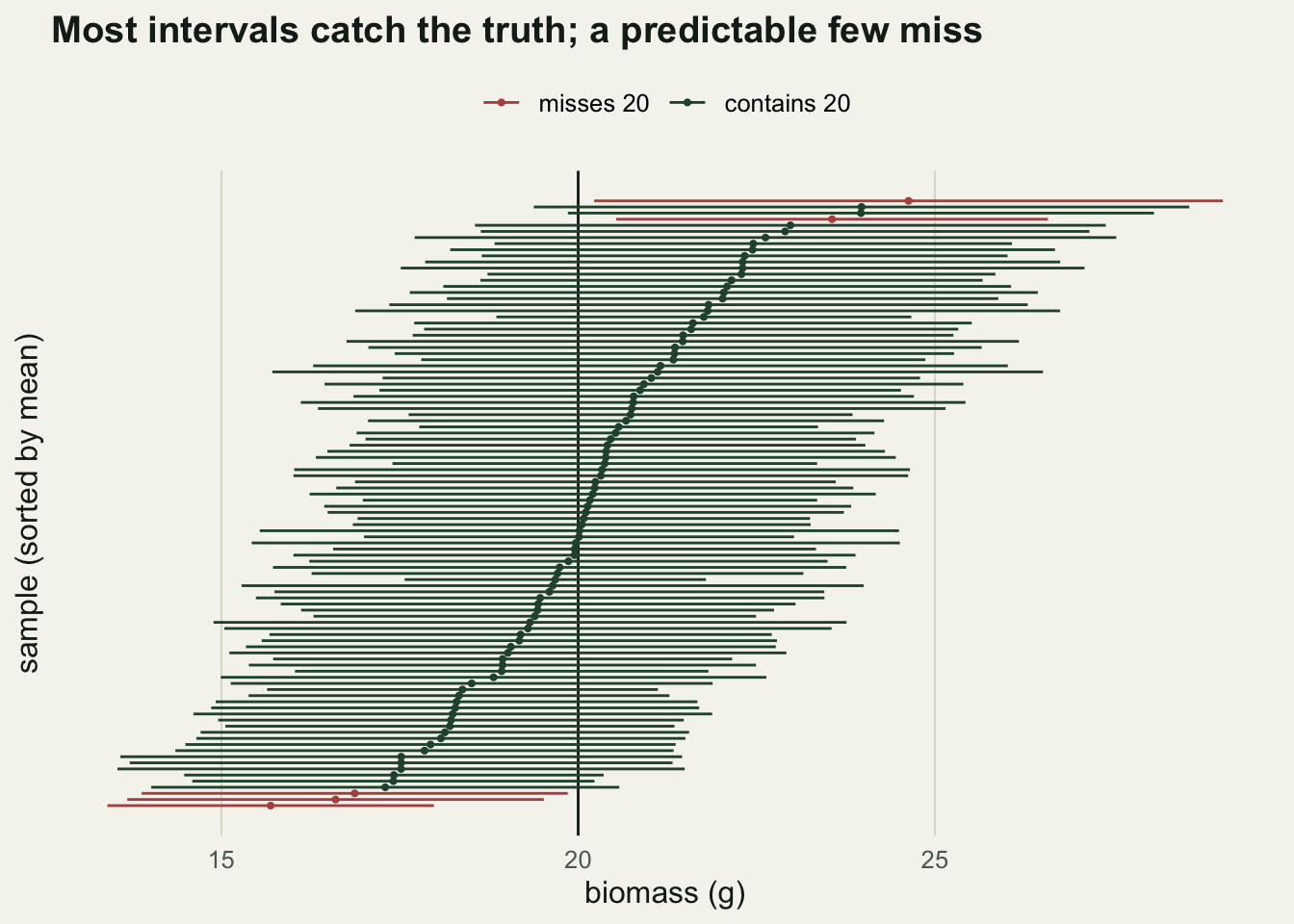

Figure 2: One hundred 95% confidence intervals from one hundred independent samples of n = 30. Each segment is one interval; the vertical line is the true mean. Five intervals miss it, matching the nominal 5% miss rate.

Proportions need a better interval

Counts and proportions are everywhere in ecology: occupied sites, infected hosts, germinated seeds. The obvious interval, \(\hat{p} \pm 1.96\sqrt{\hat{p}(1-\hat{p})/n}\), is the Wald interval, and it misbehaves badly near 0 and 1. Suppose 3 of 25 sites are occupied.

x_occ <- 3; n_site <- 25
phat <- x_occ / n_site

wald   <- phat + c(-1, 1) * qnorm(0.975) * sqrt(phat * (1 - phat) / n_site)
wilson <- as.numeric(prop.test(x_occ, n_site, correct = FALSE)$conf.int)

round(c(p_hat = phat, wald_lo = wald[1], wald_hi = wald[2],
        wilson_lo = wilson[1], wilson_hi = wilson[2]), 3)

    p_hat   wald_lo   wald_hi wilson_lo wilson_hi 
    0.120    -0.007     0.247     0.042     0.300 

The estimate is 0.12. The Wald interval runs down to -0.007, a negative proportion, which is impossible. The Wilson interval from prop.test() stays inside [0, 1] at 0.042 to 0.3 and keeps its coverage near nominal even for small counts. For proportions, reach for the Wilson interval (or an exact method) and leave Wald for large samples well away from the boundaries.

What to carry forward

Report the standard error or a confidence interval, not the standard deviation, when the claim is about a mean or a model coefficient: readers want the precision of your estimate, not the variability of individual organisms. Read a confidence interval as a statement about the procedure, not a probability attached to the one interval you happened to compute. Treat the nominal level as a target to verify: small samples and skew can erode it, and a few lines of simulation will tell you by how much. For proportions, use an interval that respects the [0, 1] boundary. None of this requires a package beyond base R, and all of it travels directly from these synthetic plots to real field data.

References

Cumming G 2014 Psychological Science 25(1):7-29 (10.1177/0956797613504966)

Brown LD, Cai TT, DasGupta A 2001 Statistical Science 16(2):101-133 (10.1214/ss/1009213286)

Crawley MJ 2013 The R Book, 2nd edn. Wiley. ISBN 9780470973929

Related tutorials

• Bootstrap confidence intervals
• A reproducible statistical workflow
• Publication-quality ggplot figures