library(boot)
library(vegan)
library(ggplot2)

paper <- "#f5f4ee"; ink <- "#16241d"; forest <- "#275139"
gold  <- "#cda23f"; miss_red <- "#b5534e"; faint <- "#5d6b61"; line <- "#dad9ca"

theme_te <- theme_minimal(base_size = 12) +
  theme(panel.grid.minor = element_blank(),
        panel.grid.major = element_line(colour = line, linewidth = 0.3),
        plot.background = element_rect(fill = paper, colour = NA),
        panel.background = element_rect(fill = paper, colour = NA),
        axis.title = element_text(colour = ink),
        axis.text = element_text(colour = faint),
plot.title = element_text(colour = ink, face = "bold"))Bootstrap confidence intervals in R
statistics
bootstrap
ecology tutorial
R
Bootstrap confidence intervals in R when no formula applies: percentile and BCa methods on a Shannon index and a regression slope, and where it breaks.
The standard confidence interval needs a formula for the standard error, and that formula needs an assumption about the sampling distribution, usually normality delivered by the central limit theorem. For a mean that assumption is fine. For a Shannon diversity index, a median, a ratio of two counts, or a regression slope built on skewed residuals, there is often no clean formula and no reason to trust the normal approximation. The bootstrap sidesteps both problems. It replaces the missing theory with brute force: resample the data you have, recompute the statistic thousands of times, and read the confidence interval off the spread of those replicates.
The idea is that your sample stands in for the population. Drawing a new sample of the same size from your data with replacement mimics drawing a fresh sample from the population, so the variation across those resamples approximates the sampling variation you cannot observe directly. We use the boot package, which ships with R, and walk through one statistic that has no tidy interval, one that does, and one case where the bootstrap quietly fails.
A statistic with no formula: Shannon diversity
Take one sampled assemblage of 286 individuals sorted into eight species. The Shannon index summarises its diversity, but its sampling distribution has no convenient closed form, so a textbook interval is not available. Resample the individuals instead.
counts <- c(120, 64, 38, 25, 17, 11, 7, 4)     # abundance of 8 species
species_vec <- rep(seq_along(counts), counts)   # one entry per individual

shannon <- function(v) {
  p <- table(v) / length(v)
  -sum(p * log(p))
}
H_obs <- shannon(species_vec)

boot_stat <- function(d, i) shannon(d[i])       # statistic on a resample
set.seed(501)
bA <- boot(species_vec, boot_stat, R = 3000)
ciA <- boot.ci(bA, type = c("norm", "perc", "bca"))

round(c(H_obs = H_obs, boot_SE = sd(bA$t),
        perc_lo = ciA$percent[4], perc_hi = ciA$percent[5],
        bca_lo = ciA$bca[4], bca_hi = ciA$bca[5]), 4)
H_obs boot_SE perc_lo perc_hi bca_lo bca_hi
1.6243 0.0509 1.5073 1.7053 1.5358 1.7269 The observed index is 1.624. The bootstrap standard error, simply the standard deviation of the 3000 replicate indices, is 0.051. From the replicate distribution boot.ci() returns several intervals. The percentile interval just takes the 2.5th and 97.5th percentiles of the replicates, here 1.507 to 1.705. The BCa interval (bias-corrected and accelerated) adjusts for two things the percentile method ignores: a median bias in the replicates and a skew that changes with the parameter value. It lands at 1.536 to 1.727, nudged upward here because resampling individuals tends to lose rare species and pull diversity estimates slightly down, a bias BCa partly repairs.
boot_df <- data.frame(H = bA$t)
ggplot(boot_df, aes(H)) +
  geom_histogram(bins = 40, fill = forest, colour = paper, linewidth = 0.2) +
  geom_vline(xintercept = H_obs, colour = ink, linewidth = 0.8) +
  geom_vline(xintercept = c(ciA$percent[4], ciA$percent[5]),
             colour = gold, linewidth = 0.7, linetype = "dashed") +
  geom_vline(xintercept = c(ciA$bca[4], ciA$bca[5]),
             colour = miss_red, linewidth = 0.7, linetype = "dotted") +
  labs(x = "bootstrapped Shannon index", y = "replicate count",
       title = "Bootstrap distribution of Shannon diversity") +
  theme_te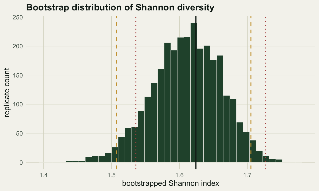
A statistic that has a formula, stress-tested
A regression slope does have a standard interval, but it assumes roughly normal residuals. When the noise is skewed, the bootstrap is a useful second opinion. Here species richness rises along a gradient with a true slope of 0.8 and strongly right-skewed errors. Rather than resample residuals, we resample whole rows, the pairs of x and y, which makes no assumption about the error shape.
set.seed(77)
ndat <- 40
x <- runif(ndat, 0, 10)
err <- (rexp(ndat, rate = 1) - 1) * 2.2        # skewed, centred near zero
y <- 2 + 0.8 * x + err                          # true slope = 0.8
dat <- data.frame(x, y)

ols <- lm(y ~ x, dat)

slope_stat <- function(d, i) coef(lm(y ~ x, d[i, ]))["x"]
set.seed(909)
bB <- boot(dat, slope_stat, R = 3000)
ciB <- boot.ci(bB, type = c("perc", "bca"))

round(c(ols_slope = coef(ols)["x"],
        ols_lo = confint(ols)["x", 1], ols_hi = confint(ols)["x", 2],
        boot_SE = sd(bB$t),
        bca_lo = ciB$bca[4], bca_hi = ciB$bca[5]), 4)
ols_slope.x ols_lo ols_hi boot_SE bca_lo bca_hi
0.6655 0.4109 0.9201 0.1312 0.3498 0.8694 The normal-theory interval runs from 0.411 to 0.92, and the BCa bootstrap interval from 0.35 to 0.869. Both contain the true 0.8, and they are close, which is itself the lesson: with 40 points the central limit theorem rescues the classical interval even though the errors are skewed, and the bootstrap confirms it while leaning slightly wider. When the two disagree, trust the bootstrap, because it is the one not relying on an assumption the data may violate.
When the bootstrap fails
The bootstrap is not magic. It struggles for statistics that depend on the extreme order statistics, because a resample can never contain a value larger than the largest one you observed. Bootstrapping the maximum makes this vivid.
set.seed(31)
samp <- rgamma(30, 4, 0.2)
max_stat <- function(d, i) max(d[i])
set.seed(32)
bMax <- boot(samp, max_stat, R = 3000)

c(observed_max = round(max(samp), 2),
  distinct_bootstrap_values = length(unique(bMax$t)))
observed_max distinct_bootstrap_values
63.65 8.00 maxdf <- data.frame(m = bMax$t)
ggplot(maxdf, aes(m)) +
geom_histogram(bins = 40, fill = miss_red, colour = paper, linewidth = 0.2) +
geom_vline(xintercept = max(samp), colour = ink, linewidth = 0.8) +
labs(x = "bootstrapped maximum", y = "replicate count",
title = "A statistic the bootstrap cannot handle") +
theme_te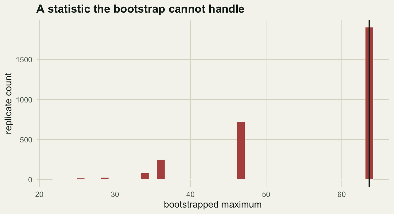
Only 8 distinct values appear across 3000 resamples, every one at or below the observed maximum of 63.7. The distribution is truncated by construction, and any interval read from it is meaningless. The same caution applies, less dramatically, to minima, ranges, and any sample size small enough that a few influential points dominate every resample.
What to carry forward
Reach for the bootstrap when the statistic has no standard error formula, or when it has one that rests on an assumption your data break. Resample the natural unit: individuals for a pooled diversity index, whole rows for a regression, plots for a community-level summary. Prefer the BCa interval over the plain percentile interval, since it corrects for bias and skew at little extra cost, and use a few thousand resamples so the percentiles are stable. Keep its limits in mind: the bootstrap cannot invent data beyond what you observed, so it fails for extreme order statistics and gets shaky at very small sample sizes. Within those bounds it turns a hard theoretical problem into a short, honest computation.
References
Efron B, Tibshirani RJ 1993 An Introduction to the Bootstrap. Chapman and Hall. ISBN 9780412042317
DiCiccio TJ, Efron B 1996 Statistical Science 11(3):189-228 (10.1214/ss/1032280214)
Davison AC, Hinkley DV 1997 Bootstrap Methods and their Application. Cambridge University Press. ISBN 9780521574716