library(ggplot2)
qgev <- function(p, mu, sigma, xi) {
  if (abs(xi) < 1e-6) return(mu - sigma * log(-log(p)))
  mu + (sigma / xi) * ((-log(p))^(-xi) - 1)
}
rgev <- function(n, mu, sigma, xi) qgev(runif(n), mu, sigma, xi)
nll_gev <- function(par, x) {
  mu <- par[1]; sigma <- exp(par[2]); xi <- par[3]; z <- (x - mu) / sigma
  if (abs(xi) < 1e-6) { ll <- -log(sigma) - z - exp(-z) }
  else {
    t <- 1 + xi * z
    if (any(!is.finite(t)) || any(t <= 0)) return(1e10)
    ll <- -log(sigma) - (1 / xi + 1) * log(t) - t^(-1 / xi)
  }
  v <- -sum(ll); if (!is.finite(v)) return(1e10); v
}

set.seed(4246)
ymax <- rgev(60, 31.0, 1.6, 0.13)
s0 <- sd(ymax) * sqrt(6) / pi
opt <- optim(c(mean(ymax) - 0.5772 * s0, log(s0), 0.1), nll_gev,
             x = ymax, method = "BFGS", hessian = TRUE)
stopifnot(opt$convergence == 0)   # check before inverting the Hessian
mu <- opt$par[1]; sigma <- exp(opt$par[2]); xi <- opt$par[3]
cov_nat <- diag(c(1, sigma, 1)) %*% solve(opt$hessian) %*% diag(c(1, sigma, 1))
return_level <- function(m) qgev(1 - 1 / m, mu, sigma, xi)Return levels and uncertainty
R
extreme value theory
statistics
ecology tutorial
Honest intervals on extreme value return levels in R with profile likelihood, why the delta method is too narrow, and a trend with non-stationary GEV.
Corrected 14 October 2026: the section on the shape parameter said the return level inherits almost all of its uncertainty from the shape; in the post’s own delta-method variance the shape carries most of it but not almost all, and the sentence now says most.
Corrected 30 September 2026: the closing section said the old design event could become a much more frequent one from one decade to the next; in this example that shift took the whole record, and the sentence now says so.
The two previous posts fitted extreme value models and read a return level off each: the GEV from annual maxima, the GPD from threshold exceedances. Both gave a single number for the hundred-year event. A single number is where the trouble starts. The return level is an extrapolation to a return period beyond the length of the record, steered by a shape parameter that a short series barely constrains, and its uncertainty is both large and lopsided. This post is about putting an honest interval on it.
Two things make return level uncertainty awkward. First, the usual symmetric confidence interval, from the delta method, is the wrong shape: the sampling distribution of a high quantile is skewed, and a symmetric interval understates how far the level can reach upward. Second, the interval is dominated by the shape parameter, so it widens fast as the return period grows. We build both the naive and the honest interval by hand, then face what a trend does to the whole idea of a return period.
The return level and a first, symmetric interval
Recall the \(m\)-observation return level: the value exceeded on average once every \(m\) blocks. For a GEV it is the \((1 - 1/m)\) quantile,
\[z_m = \mu - \frac{\sigma}{\xi}\left[1 - \{-\log(1 - 1/m)\}^{-\xi}\right],\]
which our quantile function returns directly. We reuse the sixty annual maxima from the block maxima post so the numbers line up.
The fit gives a shape of 0.060 with a standard error of 0.081. The hundred-year return level is 39.73. The delta method turns the parameter covariance into a variance for \(z_m\) through its gradient, \(\text{Var}(z_m) \approx \nabla z_m^\top \Sigma \nabla z_m\), and hands back a symmetric interval.
grad_zm <- function(m) {
  y <- -log(1 - 1 / m)
  c(1,
    -(1 / xi) * (1 - y^(-xi)),
    (sigma / xi^2) * (1 - y^(-xi)) - (sigma / xi) * y^(-xi) * log(y))
}
delta_ci <- function(m) {
  g <- grad_zm(m)
  v <- as.numeric(t(g) %*% cov_nat %*% g)
  est <- return_level(m)
  c(est = est, lo = est - 1.96 * sqrt(v), hi = est + 1.96 * sqrt(v))
}
d100 <- delta_ci(100)
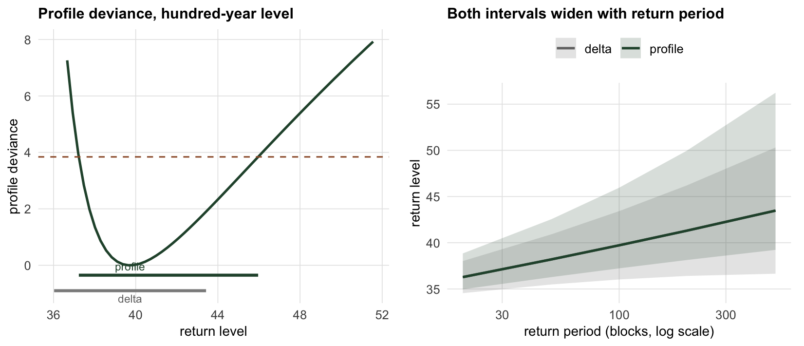
The delta interval for the hundred-year level runs from 36.03 to 43.42, symmetric about the estimate by construction. That symmetry is the problem. Pushing the shape parameter up sends the return level up by more than the same drop in the shape pulls it down, so the real interval should reach further above the estimate than below. A symmetric interval cannot show that.
The honest interval: profile likelihood
The fix is to build the interval from the likelihood itself rather than from a quadratic approximation to it. Reparameterise the GEV so the return level is one of its parameters: solve the return level formula for \(\mu\),
\[\mu = z_m - \frac{\sigma}{\xi}\left[\{-\log(1 - 1/m)\}^{-\xi} - 1\right],\]
and substitute it back. The log-likelihood is now a function of \(z_m\), \(\sigma\) and \(\xi\). Fixing \(z_m\) and maximising over the other two gives the profile log-likelihood, and the set of \(z_m\) values for which the profile deviance stays below the chi-squared cutoff is the confidence interval.
prof_ll <- function(zm, m) {
  y <- -log(1 - 1 / m)
  obj <- function(theta) {
    sg <- exp(theta[1]); xn <- theta[2]
    mu_z <- zm - (sg / xn) * (y^(-xn) - 1)
    nll_gev(c(mu_z, log(sg), xn), ymax)
  }
  r <- tryCatch(optim(c(log(sigma), xi), obj, method = "Nelder-Mead"),
                error = function(e) NULL)
  if (is.null(r)) return(-1e10)
  -r$value
}
profile_ci <- function(m, span = 25, k = 241) {
  zhat <- return_level(m); Lmax <- -opt$value
  zg <- seq(zhat - span, zhat + span * 1.6, length.out = k)
  dev <- 2 * (Lmax - sapply(zg, prof_ll, m = m))
  crit <- qchisq(0.95, 1)
  ok <- which(dev <= crit)
  lo <- approx(dev[c(min(ok) - 1, min(ok))], zg[c(min(ok) - 1, min(ok))], crit)$y
  hi <- approx(dev[c(max(ok), max(ok) + 1)], zg[c(max(ok), max(ok) + 1)], crit)$y
  list(est = zhat, lo = lo, hi = hi, zg = zg, dev = dev, crit = crit)
}
p100 <- profile_ci(100)
The profile interval for the hundred-year level runs from 37.23 to 45.96. Compare the two. The delta interval reached 3.70 above the estimate and 3.70 below, the same on each side. The profile interval reaches 6.23 above and only 2.50 below. The upper end is where the honesty is: the hundred-year temperature could plausibly be more than four degrees above our point estimate, a possibility the symmetric interval quietly hides.
Why the shape parameter runs the show
The return level inherits most of its uncertainty from the shape. Hold the location and scale at their estimates and move the shape by a single standard error in each direction.
se_xi <- sqrt(cov_nat[3, 3])
z_lo <- qgev(1 - 1 / 100, mu, sigma, xi - se_xi)
z_mid <- qgev(1 - 1 / 100, mu, sigma, xi)
z_hi <- qgev(1 - 1 / 100, mu, sigma, xi + se_xi)
A shape one standard error below the estimate gives a hundred-year level of 38.20; one standard error above gives 41.70, against 39.73 at the estimate. A swing of more than three degrees in the design temperature follows from a change in the shape that the data cannot even rule out. This is why the interval widens so fast with the return period: the further out the level, the more it is a pure function of the shape, and the shape is the parameter a short series holds most weakly. The right panel above makes it concrete: the five-hundred-year level in this fit could sit anywhere across a range of many degrees.
When there is a trend: non-stationary GEV
Every return level so far assumed the climate that produced the maxima is the climate that will produce the next ones. Under a warming trend that assumption fails, and the return period, a fixed recurrence rate, stops being well defined. The GEV handles this by letting a parameter depend on a covariate. The simplest useful form makes the location a linear function of time, \(\mu(t) = \beta_0 + \beta_1 t\), holding the scale and shape fixed.
nll_ns <- function(par, y, t) {
  b0 <- par[1]; b1 <- par[2]; sg <- exp(par[3]); xn <- par[4]
  mu_t <- b0 + b1 * t; z <- (y - mu_t) / sg
  if (abs(xn) < 1e-6) { ll <- -log(sg) - z - exp(-z) }
  else {
    s <- 1 + xn * z
    if (any(!is.finite(s)) || any(s <= 0)) return(1e10)
    ll <- -log(sg) - (1 / xn + 1) * log(s) - s^(-1 / xn)
  }
  v <- -sum(ll); if (!is.finite(v)) return(1e10); v
}

set.seed(555)
Tn <- 80; tt <- 0:(Tn - 1)
yt <- rgev(Tn, 30 + 0.03 * tt, 1.5, 0.1)       # a genuine warming trend
o_ns <- optim(c(30, 0, log(1.5), 0.1), nll_ns, y = yt, t = tt,
              method = "BFGS", hessian = TRUE)
stopifnot(o_ns$convergence == 0)   # check before inverting the Hessian
se_ns <- sqrt(diag(solve(o_ns$hessian)))
b0 <- o_ns$par[1]; b1 <- o_ns$par[2]
sg_ns <- exp(o_ns$par[3]); xi_ns <- o_ns$par[4]
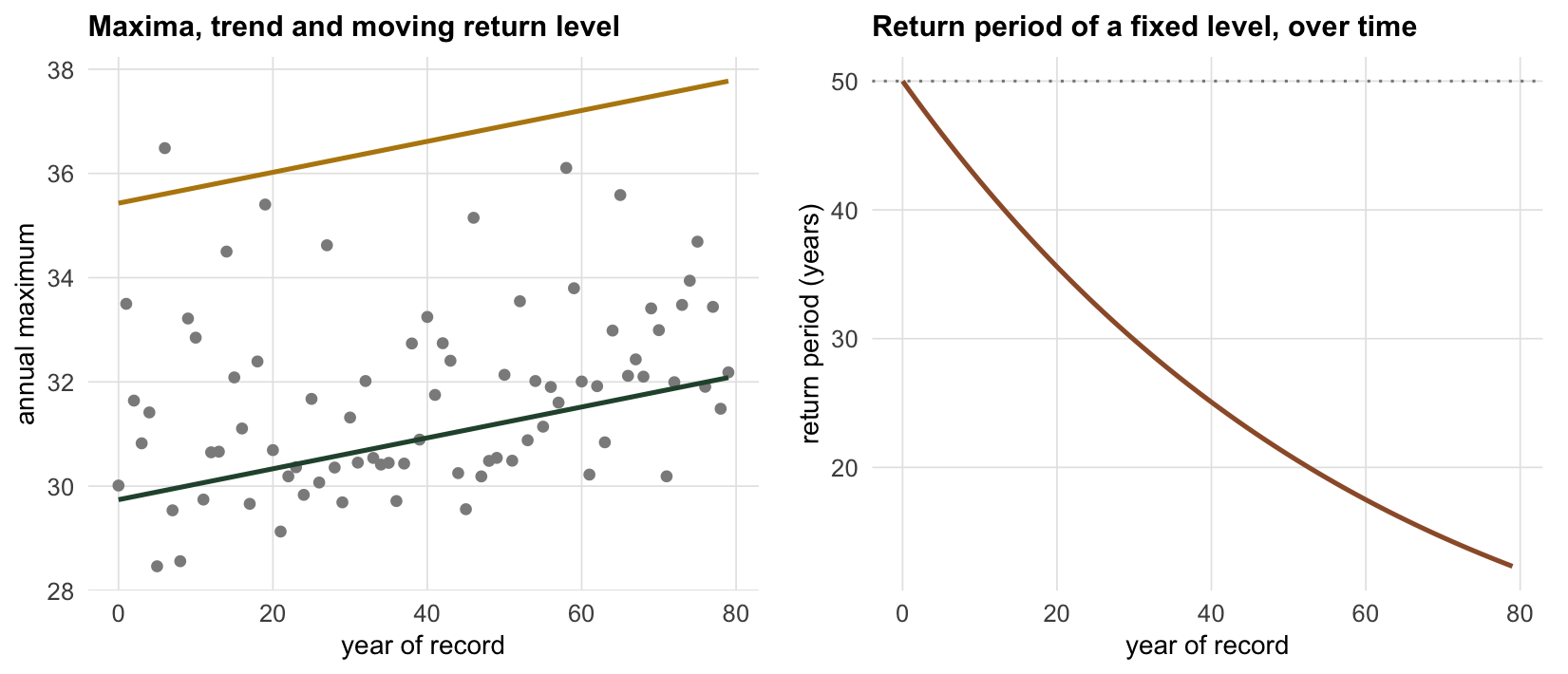
The non-stationary fit puts a slope on the location: the slope is 0.0297 per year with a standard error of 0.0058, a \(z\) of about 5.1, so the location climbs by ten times that slope each decade. The fifty-year return level is now a moving target. Computing it at the start and end of the record:
rl_year <- function(year) qgev(1 - 1 / 50, b0 + b1 * year, sg_ns, xi_ns)
z_start <- rl_year(0)
z_end <- rl_year(Tn - 1)

# the start-of-record 50-year level, seen at the end of the record
mu_end <- b0 + b1 * (Tn - 1)
s_end <- 1 + xi_ns * (z_start - mu_end) / sg_ns
p_exceed_end <- 1 - exp(-s_end^(-1 / xi_ns))
The fifty-year level rises from 35.43 at the start of the record to 37.77 at the end, a shift of 2.34 degrees. Read the other way round, the effect is starker. A temperature that was a fifty-year event at the start of the record has an annual exceedance probability of 0.081 by the end, which is a return period of about 12 years. The one-in-fifty event has become a one-in-twelve event over a single lifetime of data, purely from the trend. Under non-stationarity the phrase “the fifty-year flood” needs a date attached, and a stationary analysis that omits the trend will badly understate how often the old extreme now recurs.
One numerical caution worth flagging. The maximum likelihood machinery here rests on standard regularity conditions, and Smith (1985) showed they fail when the shape is very negative, below \(-1/2\): the usual standard errors and the chi-squared calibration of the profile likelihood are then unreliable. Ecological maxima rarely sit that far into the bounded regime, but a fit that returns a shape near or below \(-1/2\) is a signal to stop trusting the automatic intervals.
What to take away
A return level without an interval is close to meaningless, and the interval has to be the right shape. The delta method gives a symmetric interval that understates the upward reach, because the sampling distribution of a high quantile is skewed; the profile likelihood gives the honest, asymmetric interval and costs only a reparametrisation and a short search. Whichever you use, the width is governed by the shape parameter, so it grows quickly with the return period, and a long return level from a short series carries enormous uncertainty. And once there is a trend, the return period is no longer a fixed property of the system: the fifty-year event at the start of an eighty-year record can be a twelve-year event by its end, and a non-stationary fit is the only way to say so. The final post puts the whole workflow under scrutiny, checking the fit and testing how far these conclusions survive changes to the threshold, the block and the assumption of a stable climate.
References
Coles, S. 2001. An Introduction to Statistical Modeling of Extreme Values. Springer (ISBN 978-1-85233-459-8).
Smith, R.L. 1985. Biometrika 72(1):67-90 (10.1093/biomet/72.1.67).
Katz, R.W., Parlange, M.B. and Naveau, P. 2002. Advances in Water Resources 25(8-12):1287-1304 (10.1016/S0309-1708(02)00056-8).
Coles, S., Pericchi, L.R. and Sisson, S. 2003. Journal of Hydrology 273(1-4):35-50 (10.1016/S0022-1694(02)00353-0).