Peaks over threshold and the GPD

Keep every value above a high threshold instead of one maximum per block, fit the generalised Pareto distribution by hand in R, choose the threshold, and decluster dependent extremes.

The block maxima approach keeps one value per block and throws the rest away. That is wasteful. If the two hottest days of a year both exceed anything seen in the previous decade, block maxima records only one of them and discards the other. A long daily record might hold a few hundred genuine extremes, yet a sixty-year block-maxima analysis reduces it to sixty numbers, and we saw what that does to the shape parameter: it is barely identified.

The peaks-over-threshold (POT) approach keeps every observation above a high threshold. From a daily record it can extract several hundred exceedances rather than a few dozen maxima, and that alone sharpens the tail. This post fits the distribution those exceedances follow, the generalised Pareto, entirely in base R, then confronts the two problems POT introduces in place of the block size: where to put the threshold, and what to do when extremes arrive in clusters.

The distribution of threshold excesses

Fix a high threshold \(u\) and look only at the excesses \(Y = X - u\) for observations with \(X > u\). There is a theorem, due to Pickands (1975) and Balkema and de Haan (1974), that plays the same role for excesses that the extremal types theorem played for maxima: as the threshold rises, the excess distribution converges to the generalised Pareto distribution (GPD), whatever the underlying data. Its distribution function is

\[H(y) = 1 - \left(1 + \xi\,\frac{y}{\sigma}\right)^{-1/\xi}, \qquad y > 0,\; 1 + \xi y/\sigma > 0,\]

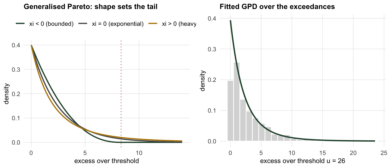
with scale \(\sigma > 0\) and shape \(\xi\). The shape is the same \(\xi\) as in the GEV, and it plays the same role. A positive \(\xi\) gives a heavy tail with no upper limit; \(\xi = 0\) gives the exponential (the light-tailed case, read as a limit); a negative \(\xi\) gives a tail with a finite upper endpoint at \(-\sigma/\xi\). If block maxima of a process follow a GEV with shape \(\xi\), its threshold excesses follow a GPD with the very same shape. The two approaches estimate the same tail; they differ in how much data they use to do it.

As before, base R has no GPD functions, so we write them.

library(ggplot2)
dgpd <- function(y, sigma, xi) {
  if (abs(xi) < 1e-8) return((1 / sigma) * exp(-y / sigma))
  t <- 1 + xi * y / sigma
  out <- numeric(length(y)); ok <- t > 0 & y >= 0
  out[ok] <- (1 / sigma) * t[ok]^(-1 / xi - 1)
  out
}
qgpd <- function(p, sigma, xi) {
  if (abs(xi) < 1e-8) return(-sigma * log(1 - p))
  (sigma / xi) * ((1 - p)^(-xi) - 1)
}
rgpd <- function(n, sigma, xi) qgpd(runif(n), sigma, xi)

Fitting the GPD to exceedances

Consider a daily environmental variable recorded for roughly twenty-two years, eight thousand observations. This could be daily maximum temperature, river discharge or significant wave height; the point of interest is the upper tail. We simulate a record whose upper tail is genuinely generalised Pareto above a reference level, then recover it.

set.seed(4247)
n <- 8000
u0 <- 25; sigma0 <- 2.5; xi0 <- 0.15    # true tail above the reference level u0
is_tail <- runif(n) < 0.10
draws <- numeric(0)                       # bulk: Normal(20, 3) truncated below u0
while (length(draws) < sum(!is_tail)) {
  cand <- rnorm(sum(!is_tail), 20, 3)
  draws <- c(draws, cand[cand < u0])
}
x <- numeric(n)
x[!is_tail] <- draws[seq_len(sum(!is_tail))]
x[is_tail]  <- u0 + rgpd(sum(is_tail), sigma0, xi0)

The negative log-likelihood is a direct transcription of the GPD density, with the scale on the log scale to keep it positive. We fit at a threshold of 26.

nll_gpd <- function(par, y) {
  sigma <- exp(par[1]); xi <- par[2]
  if (abs(xi) < 1e-8) return(length(y) * log(sigma) + sum(y) / sigma)
  t <- 1 + xi * y / sigma
  if (any(t <= 0)) return(1e10)
  length(y) * log(sigma) + (1 / xi + 1) * sum(log(t))
}
fit_gpd <- function(y) {
  o <- optim(c(log(mean(y)), 0.1), nll_gpd, y = y,
             method = "BFGS", hessian = TRUE)
  se <- sqrt(diag(solve(o$hessian)))
  list(sigma = exp(o$par[1]), xi = o$par[2], se_xi = se[2], nexc = length(y))
}

u  <- 26
exc <- x[x > u] - u
fit <- fit_gpd(exc)
xi_lo <- fit$xi - 1.96 * fit$se_xi
xi_hi <- fit$xi + 1.96 * fit$se_xi

The threshold of 26 leaves 559 exceedances, and the fit returns a scale of 2.54 and a shape of 0.157 with a standard error of 0.054. The Wald interval for the shape runs from 0.05 to 0.26, which excludes zero and sits close to the true value of 0.15. This is the payoff over block maxima. With sixty annual maxima the shape came out with a standard error near 0.08 and an interval that swallowed zero and a wide band of negative values; here, with 559 exceedances drawn from the same tail, the standard error is roughly half that and the tail is clearly identified as heavy. Same \(\xi\), far more information, because we kept the extremes the block maxima approach would have thrown away.

Figure 1: The generalised Pareto distribution. Left: three densities sharing a scale but differing in shape, with the negative-shape case ending at a finite bound (dotted line). Right: the fitted GPD density over the threshold excesses.

Choosing the threshold

The block size was the awkward choice of the last post; the threshold is its replacement here, and it carries the same bias-variance tension. Too low and the GPD limit has not kicked in, so the fit is biased by the body of the distribution. Too high and only a handful of exceedances remain, so the variance explodes. There is no formula that returns the right threshold. What there are, are two diagnostic plots that show the range over which the choice is defensible.

The first is the mean residual life plot. If the excesses over \(u\) are GPD with shape \(\xi < 1\), the mean excess is a linear function of the threshold,

\[E[X - u \mid X > u] = \frac{\sigma_u}{1 - \xi} = \frac{\sigma_{u_0} + \xi(u - u_0)}{1 - \xi},\]

so above the level where the GPD holds, the sample mean excess should trace a straight line. Below that level it bends. We look for the lowest threshold past which the plot is roughly linear.

us <- seq(21, 32, by = 0.5)
mrl <- t(sapply(us, function(uu) {
  e <- x[x > uu] - uu
  c(mean = mean(e), se = sd(e) / sqrt(length(e)))
}))
mrl <- data.frame(u = us, mrl)

The second is the parameter stability plot. Refit the GPD across a grid of thresholds and plot the shape estimate with its confidence interval. Because the GPD shape does not change as the threshold rises (a GPD tail is still GPD above any higher level), the estimates should be stable, within their widening intervals, above the point where the limit holds.

uu_grid <- seq(23, 31, by = 1)
stab <- t(sapply(uu_grid, function(uu) {
  g <- fit_gpd(x[x > uu] - uu)
  c(u = uu, xi = g$xi, lo = g$xi - 1.96 * g$se_xi, hi = g$xi + 1.96 * g$se_xi)
}))
stab <- as.data.frame(stab)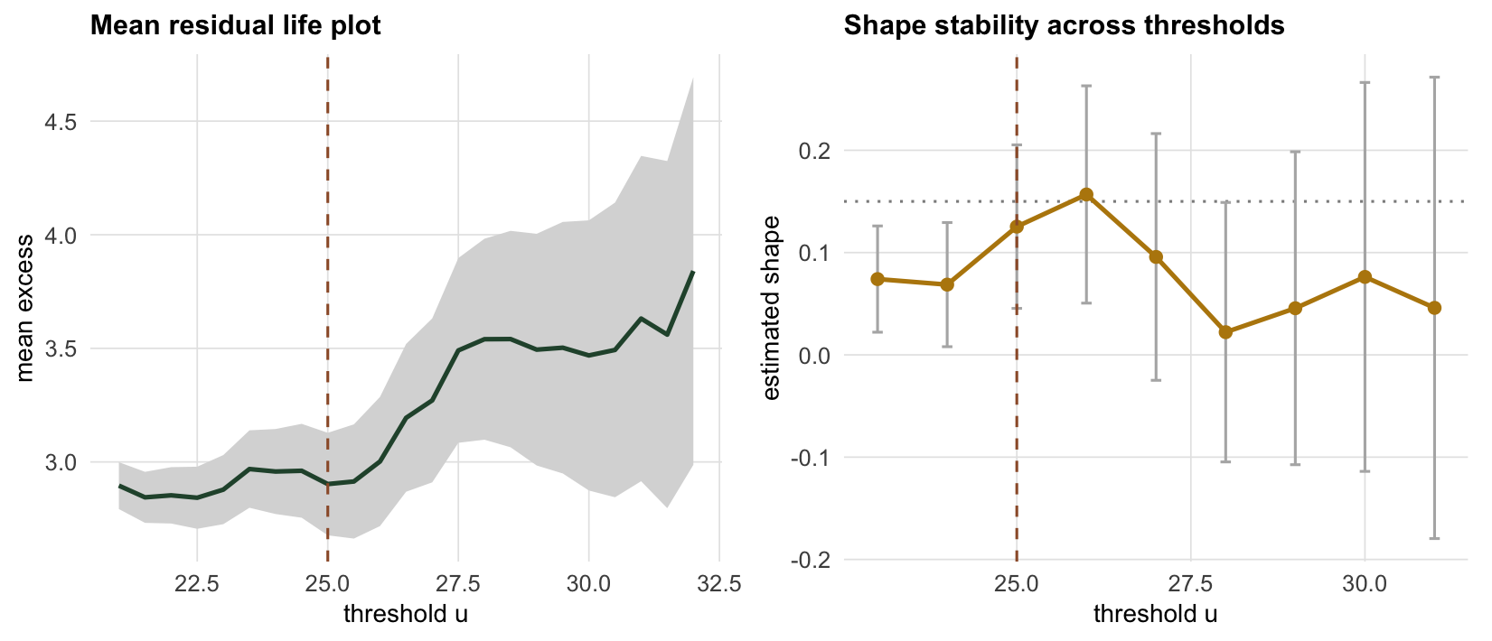

Figure 2: Threshold diagnostics. Left: the mean residual life plot, flat through the body and turning to a rising line once the generalised Pareto tail takes over near 25. Right: the shape estimate is stable within its widening intervals above the same level, with no threshold standing out as objectively correct.

Both plots point at a threshold somewhere around 25 to 26: low enough to keep a useful number of exceedances, high enough that the GPD approximation has taken hold. Neither singles out one value. The honest reading is that the threshold is a knob, and a careful analysis reports how the answer moves as it turns, rather than pretending a single setting is correct.

From the fit to a return level

A GPD fit becomes a design number through the return level, exactly as the GEV fit did, with one extra ingredient: the rate at which the threshold is exceeded. Writing \(\zeta_u = P(X > u)\), the level exceeded on average once every \(m\) observations is

\[x_m = u + \frac{\sigma}{\xi}\left[(m\,\zeta_u)^{\xi} - 1\right].\]

With daily data, an \(N\)-year level uses \(m = 365N\).

zeta <- mean(x > u)
return_level <- function(years) {
  m <- years * 365
  u + (fit$sigma / fit$xi) * ((m * zeta)^fit$xi - 1)
}
rl10  <- return_level(10)
rl100 <- return_level(100)

The exceedance rate is 0.0699, so on the order of 26 exceedances a year. The estimated ten-year level is 48.4 and the hundred-year level is 65.2, against true values near 48.9 and 65.6. The estimates are close because this fit pinned down the shape. The next post takes the return level seriously as a quantity with its own, often uncomfortable, uncertainty; here it is enough to see that POT reaches it through the same door as block maxima, with the exceedance rate carrying the extra bookkeeping.

When extremes cluster: declustering

There is one assumption in all of the above that ecological and environmental series routinely break: that exceedances are independent. A heatwave is several hot days in a row, not one. A flood keeps a river above its banks for a week. When the process is serially dependent, exceedances arrive in clusters, and treating every one as an independent draw counts the same episode many times over. The likelihood then reports a sample size larger than the number of genuinely independent extremes, and the standard errors come out too small, a false precision of exactly the kind the post on bootstrapping dependent data warns about.

We simulate a dependent daily series by driving it with a first-order autoregressive process, so that exceedances tend to occur in runs, and give it a genuine GPD upper tail.

set.seed(9247)
m2 <- 6000; rho <- 0.6
z <- numeric(m2); z[1] <- rnorm(1)
for (t in 2:m2) z[t] <- rho * z[t - 1] + sqrt(1 - rho^2) * rnorm(1)
ud <- 2.0
pz <- pnorm(z)
xd <- ifelse(pz > 0.9, ud + rgpd(m2, 1.5, 0.12),
             qnorm(pmin(pz / 0.9, 0.999), 0, 1))   # true tail shape 0.12
exc_idx <- which(xd > ud)

The extremal index \(\theta\) measures how much the exceedances cluster: it is, loosely, the reciprocal of the mean cluster size, so \(\theta = 1\) means no clustering and small values mean long runs. The intervals estimator of Ferro and Segers (2003) computes it from the gaps between exceedance times alone, with no tuning constant.

extremal_index <- function(exc_times) {
  s <- diff(exc_times); N <- length(exc_times)
  if (max(s) <= 2) {
    theta <- 2 * sum(s)^2 / ((N - 1) * sum(s^2))
  } else {
    theta <- 2 * sum(s - 1)^2 / ((N - 1) * sum((s - 1) * (s - 2)))
  }
  min(1, theta)
}
theta_hat <- extremal_index(exc_idx)

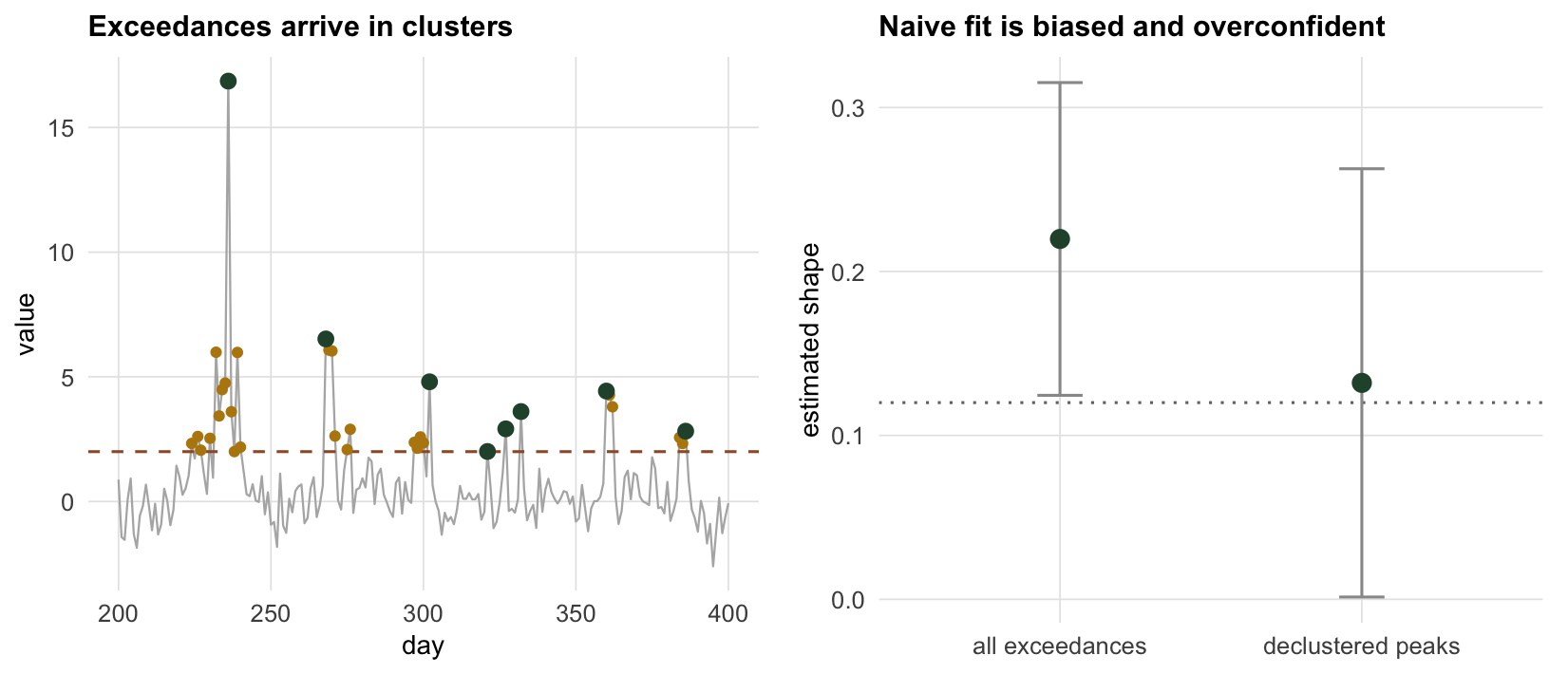
There are 695 exceedances, but the extremal index is 0.57, so barely more than half of them carry independent information. To fit the GPD honestly we decluster: split the exceedances into clusters wherever a run of non-exceedances is long enough (four here, say four calm days ending an episode), then keep only the peak of each cluster. Those peaks are close to independent, and it is them the GPD should see.

r <- 4
cluster_id <- cumsum(c(1, diff(exc_idx) > r))
n_clusters <- length(unique(cluster_id))
peaks <- as.numeric(tapply(xd[exc_idx], cluster_id, max)) - ud

fit_all  <- fit_gpd(xd[exc_idx] - ud)     # naive: every exceedance
fit_peak <- fit_gpd(peaks)                # declustered: cluster peaks only

Declustering leaves 287 cluster peaks out of the 695 raw exceedances. The difference in the fits is the whole lesson. The naive fit, treating all 695 exceedances as independent, returns a shape of 0.220 with a standard error of 0.049. The declustered fit, on 287 peaks, returns 0.132 with a standard error of 0.067. The true tail shape was 0.12. The naive fit is both biased away from the truth, pulled up by the repeated within-cluster values, and falsely confident, with a standard error too small to be believed. The declustered fit lands on the true shape and reports the wider uncertainty that 287 independent extremes actually warrant.

Figure 3: Clustering and its cost. Left: a window of the dependent series, with exceedances marked and cluster peaks highlighted; extremes arrive in runs, not singly. Right: the shape estimate and interval from the naive fit to all exceedances versus the declustered fit to cluster peaks, against the true value (dotted).

What to take away

Peaks over threshold trades the block size for the threshold and buys a large gain in efficiency: the same tail, estimated from every extreme rather than one per year, with a shape parameter that is properly identified. The generalised Pareto is the distribution those excesses must follow, and fitting it is a short likelihood. The two cautions are the ones to carry forward. The threshold is a bias-variance knob with no objective optimum; the mean residual life and parameter stability plots show the range over which a choice is defensible, and a careful analysis reports the sensitivity rather than a single number. And when extremes cluster, which in ecology they usually do, the raw exceedance count is not the independent sample size: decluster to cluster peaks, read the extremal index, and let the standard errors tell the truth. The next post takes the return level itself as the object of study and asks how far its uncertainty really stretches.

References

Pickands, J. 1975. Annals of Statistics 3(1):119-131 (10.1214/aos/1176343003).

Balkema, A.A. and de Haan, L. 1974. Annals of Probability 2(5):792-804 (10.1214/aop/1176996548).

Davison, A.C. and Smith, R.L. 1990. Journal of the Royal Statistical Society Series B 52(3):393-425 (10.1111/j.2517-6161.1990.tb01796.x).

Ferro, C.A.T. and Segers, J. 2003. Journal of the Royal Statistical Society Series B 65(2):545-556 (10.1111/1467-9868.00401).

Coles, S. 2001. An Introduction to Statistical Modeling of Extreme Values. Springer (ISBN 978-1-85233-459-8).

Related tutorials

• Block maxima and the GEV distribution
• Return levels and uncertainty
• Checking an extreme value model
• Bootstrapping dependent data