Bootstrapping dependent data: blocks and clusters

Resampling single observations destroys dependence and understates uncertainty. Use block resampling for autocorrelated series and cluster resampling for grouped data.

The ordinary bootstrap resamples individual observations, which only makes sense if the observations are interchangeable. Ecological data rarely are. Counts in successive years carry over; plots within the same site share conditions; repeated measures on the same animal move together. When you resample single observations from data like these, you shuffle away the very dependence that inflates the true uncertainty, and the bootstrap hands back a standard error that is too small and an interval that is too narrow. The fix is to resample the unit that carries the dependence: blocks of consecutive time points, or whole clusters. This post shows both failures and both repairs, on an autocorrelated series and on grouped data.

An autocorrelated series

Suppose an annual index of abundance follows a first-order autoregressive process, so each year is correlated with the last. We want a confidence interval for its long-run mean.

set.seed(2440)
phi <- 0.6; n <- 120
x <- as.numeric(arima.sim(list(ar = phi), n = n, sd = 1))   # AR(1) annual index
xbar <- mean(x)
se_iid <- sd(x) / sqrt(n)                                   # naive independence SE

With positive autocorrelation the true standard error of the mean is larger than the independence formula suggests, by roughly the square root of the variance inflation factor (1 + phi) / (1 - phi), which here is 4. So the honest standard error is about 0.23, while the naive independence value is only 0.12, half as large. The bootstrap needs to recover the larger number.

Blocks preserve the dependence

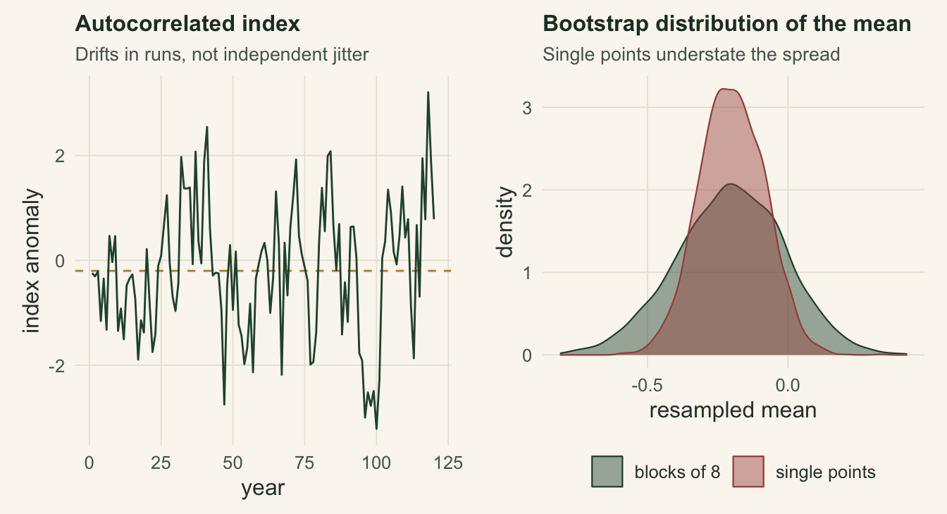
Resampling single years destroys the autocorrelation. The block bootstrap instead resamples short runs of consecutive years, so each block carries a piece of the dependence with it. We use a circular version that wraps the series end to start, which stops the endpoints from being under-represented.

set.seed(717)
B <- 3000
boot_iid <- replicate(B, mean(sample(x, n, replace = TRUE)))     # destroys dependence

cblock_mean <- function(x, l) {
  n <- length(x); k <- ceiling(n / l)
  xc <- c(x, x[seq_len(l)])                                       # wrap the series
  starts <- sample(seq_len(n), k, replace = TRUE)
  idx <- as.vector(sapply(starts, function(s) s:(s + l - 1)))[seq_len(n)]
  mean(xc[idx])
}
boot_block <- replicate(B, cblock_mean(x, 8))                     # blocks of 8 years
se_boot_iid <- sd(boot_iid); se_boot_block <- sd(boot_block)

The naive bootstrap gives a standard error of 0.12, tracking the independence formula and missing the autocorrelation entirely. The block bootstrap gives 0.19, close to the honest value. Resampling single points quietly assumed the years were independent; resampling blocks did not.

Figure 1: Left: the autocorrelated annual index, which drifts in runs rather than jittering independently. Right: the bootstrap distribution of its mean. Resampling single years (narrow) understates the spread, while resampling blocks of eight years (wide) recovers the larger, honest standard error.

Grouped data

The same failure appears whenever observations come in clusters. Suppose we sample several plots at each of a number of sites, and sites differ. Measurements from one site share its conditions, so they are positively correlated. We want the grand mean across sites.

set.seed(2441)
G <- 20; ng <- 8; N <- G * ng
mu_true <- 5; tau <- 1; sigma <- 1
gen_clustered <- function() {
  b <- rnorm(G, 0, tau)                       # site effect
  grp <- rep(seq_len(G), each = ng)
  data.frame(grp = grp, y = mu_true + b[grp] + rnorm(N, 0, sigma))
}
d <- gen_clustered()
icc <- tau^2 / (tau^2 + sigma^2)              # within-site correlation
se_naive_c <- sd(d$y) / sqrt(N)
se_true_c <- sqrt(tau^2 / G + sigma^2 / N)    # honest SE for a balanced design

The within-site correlation is 0.50, so the 160 measurements are worth far fewer independent ones. The honest standard error of the grand mean is 0.24, against a naive independence value of only 0.10.

Clusters, not rows

Resampling individual rows treats every measurement as its own independent draw. The cluster bootstrap resamples whole sites with replacement and keeps all of each chosen site’s measurements, so the between-site variation survives.

set.seed(818)
boot_row <- replicate(B, mean(sample(d$y, N, replace = TRUE)))   # resample rows

cluster_mean <- function(d, G) {
  gg <- sample(unique(d$grp), G, replace = TRUE)
  mean(unlist(lapply(gg, function(g) d$y[d$grp == g])))          # keep whole sites
}
boot_clus <- replicate(B, cluster_mean(d, G))
se_boot_row <- sd(boot_row); se_boot_clus <- sd(boot_clus)

The row bootstrap gives 0.10, matching the naive value and ignoring the clustering. The cluster bootstrap gives 0.19, close to the honest standard error. In both examples the naive bootstrap failed the same way: it resampled the wrong unit and threw the dependence away.

Does it fix the coverage?

Standard errors are one thing; interval coverage is the real test. We rebuild each study many times and check how often the 95% percentile interval traps the true value.

ar1 <- function() as.numeric(arima.sim(list(ar = phi), n = n, sd = 1))
cov_ts <- function(R = 700, Bb = 400, l = 8) {
  hi <- 0; hb <- 0
  for (r in seq_len(R)) {
    xx <- ar1()
    bi <- replicate(Bb, mean(sample(xx, n, TRUE)))
    bk <- replicate(Bb, cblock_mean(xx, l))
    hi <- hi + (0 >= quantile(bi, .025) & 0 <= quantile(bi, .975))
    hb <- hb + (0 >= quantile(bk, .025) & 0 <= quantile(bk, .975))
  }
  c(iid = hi / R, block = hb / R)
}
cov_cl <- function(R = 700, Bb = 400) {
  hr <- 0; hc <- 0
  for (r in seq_len(R)) {
    dd <- gen_clustered()
    br <- replicate(Bb, mean(sample(dd$y, N, TRUE)))
    bc <- replicate(Bb, cluster_mean(dd, G))
    hr <- hr + (mu_true >= quantile(br, .025) & mu_true <= quantile(br, .975))
    hc <- hc + (mu_true >= quantile(bc, .025) & mu_true <= quantile(bc, .975))
  }
  c(row = hr / R, cluster = hc / R)
}
set.seed(404); cts <- cov_ts()
set.seed(505); ccl <- cov_cl()
ls <- c(1, 4, 8, 12, 16, 24)
set.seed(606)
cvl <- sapply(ls, function(l) {
  h <- 0
  for (r in seq_len(500)) {
    xx <- ar1(); bk <- replicate(300, cblock_mean(xx, l))
    h <- h + (0 >= quantile(bk, .025) & 0 <= quantile(bk, .975))
  }
  h / 500
})

Figure 2: Left: coverage of the naive and dependence-aware 95% intervals in both examples. The naive intervals cover far too rarely; the block and cluster intervals recover most of the shortfall. Right: block-bootstrap coverage against block length for the series. A length of one is the naive bootstrap; coverage climbs as blocks lengthen, plateaus, then falls when blocks grow so long that too few remain. Even the best length stays a little under nominal, a reminder that block methods reduce rather than erase the problem.

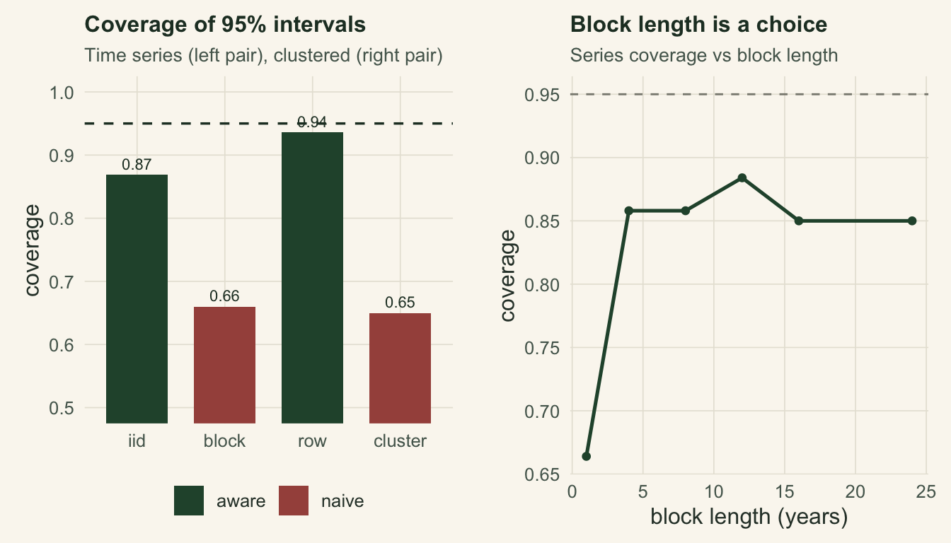
The naive intervals are badly wrong: 66% coverage for the series and 65% for the clustered data, both missing roughly a third of the time despite claiming 95%. The dependence-aware intervals recover most of the shortfall, reaching 87% and 94%. The cluster bootstrap does especially well because twenty sites give plenty of units to resample. The block bootstrap does not quite reach nominal, and the right panel shows why the choice is delicate: too short and it behaves like the naive bootstrap, too long and too few blocks remain to resample. This connects to the effective-sample-size idea from the autocorrelation tutorial, where dependence shrinks the independent information in a series.

What to take away

The bootstrap is not automatic once the data are dependent. Ask what unit carries the dependence and resample that: consecutive blocks for a time series, whole clusters for grouped data, and by extension whole subjects for repeated measures. Resampling the wrong unit, single points or single rows, silently assumes independence and understates uncertainty by a large factor, here roughly halving the standard error and dropping coverage into the sixties. The block and cluster bootstraps repair most of that, though the block length is a tuning choice and even a good one leaves a small shortfall. That last point, that a resampled interval can still miss its target, is where the next post begins: when even the right bootstrap is not enough, and how to tell.

Related tutorials

• The nonparametric bootstrap
• The parametric bootstrap
• Checking a bootstrap
• Nested counts and pseudoreplication

References

Kunsch 1989 Annals of Statistics 17(3):1217-1241 (10.1214/aos/1176347265)

Politis and Romano 1994 Journal of the American Statistical Association 89(428):1303-1313 (10.1080/01621459.1994.10476870)

Field and Welsh 2007 Journal of the Royal Statistical Society Series B 69(3):369-390 (10.1111/j.1467-9868.2007.00593.x)

Davison and Hinkley 1997 Bootstrap Methods and their Application. ISBN 978-0-521-57391-7