Checking a bootstrap: when resampling fails

The bootstrap is not automatic. See how it breaks on small samples and non-smooth statistics, why its intervals undercover, and how to check before trusting it.

The bootstrap is easy to run and easy to over-trust. Across this series it kept undercovering a little, even when it worked; and there are cases where it does not work at all, quietly returning a confident answer that is wrong. This closing post collects three ways resampling fails: when the sample is too small for the statistic to resolve, when the statistic is not smooth, and when the interval simply does not cover at the rate it claims. Each comes with the check that would have caught it.

Small samples cannot resolve a rough statistic

With few observations the bootstrap distribution is built from a limited set of resamples, and how well it fills in depends on how smooth the statistic is. Take twelve values and bootstrap two summaries: the mean and the median.

set.seed(2450)
n1 <- 12
x1 <- round(rlnorm(n1, log(20), 0.5), 1)
B <- 4000
boot_mean <- replicate(B, mean(sample(x1, n1, replace = TRUE)))
boot_med  <- replicate(B, median(sample(x1, n1, replace = TRUE)))
d_mean <- length(unique(round(boot_mean, 6)))   # distinct resampled means
d_med  <- length(unique(boot_med))              # distinct resampled medians
atom_med <- max(table(boot_med)) / B            # largest single spike

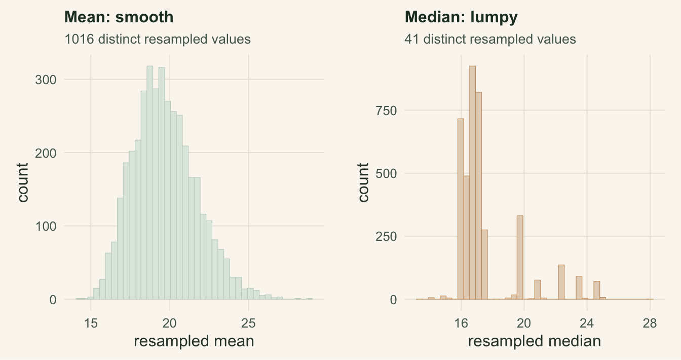
From the same twelve numbers the bootstrap mean takes 1016 distinct values, forming a smooth distribution, while the bootstrap median takes only 41, landing on a coarse lattice of order statistics with a single value carrying 9% of the resamples. The median is not smooth in the data, so at this sample size its bootstrap distribution is a handful of spikes, and any quantile read from it, including the ends of a percentile interval, can only sit on that lattice. The check is direct: look at the bootstrap distribution before trusting its tails. If it is a few tall bars rather than a filled-in shape, the interval is coarser than its decimals suggest, and you need more data or a smoother statistic.

Figure 1: Bootstrap distributions of the mean (left) and median (right) from the same twelve observations. The mean fills in smoothly; the median collapses onto a few order statistics, one of which holds nearly a tenth of all resamples. Quantiles of the right-hand distribution are quantised, so the ends of a percentile interval are coarse.

A non-smooth statistic breaks it outright

Small samples only sharpen a deeper problem: for some statistics the bootstrap is inconsistent, and no amount of data repairs it. The textbook case is the maximum of a sample from a uniform distribution, the natural estimator when the parameter is an upper bound. We draw forty values from a uniform on the interval up to one, and estimate that upper bound by the sample maximum.

set.seed(2451)
n2 <- 40; theta <- 1
x2 <- runif(n2, 0, theta)
mx <- max(x2)
boot_max <- replicate(B, max(sample(x2, n2, replace = TRUE)))
atom <- mean(boot_max == mx)                    # share of resamples pinned at the max
atom_theory <- 1 - (1 - 1/n2)^n2                # limiting value, about 0.63
ci_boot <- quantile(boot_max, c(.025, .975))    # bootstrap percentile interval
ci_exact <- c(mx, mx / (0.025)^(1/n2))          # exact interval from max/theta ~ Beta(n,1)

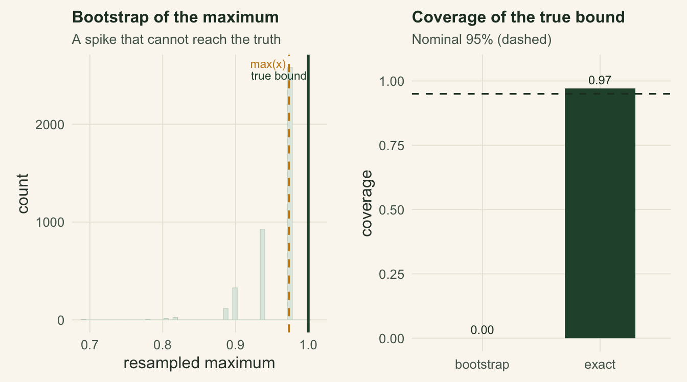
The observed maximum is 0.973. A resample includes it unless every draw misses it, so a fraction 0.65 of bootstrap maxima are exactly the observed value, matching the limiting 0.64. The bootstrap distribution is a huge spike at the maximum with a short tail below, and crucially it never exceeds the observed maximum, because resampling cannot invent a larger value. So the bootstrap interval [0.888, 0.973] sits entirely at or below the sample maximum, while the truth is above it. The exact interval, from the fact that the maximum divided by the parameter follows a known distribution, runs [0.973, 1.067] and reaches past the data as it must.

covmax <- function(R = 2000, Bb = 500) {
  hb <- 0; he <- 0
  for (r in seq_len(R)) {
    xx <- runif(n2, 0, 1); m <- max(xx)
    bb <- replicate(Bb, max(sample(xx, n2, TRUE)))
    hb <- hb + (1 >= quantile(bb, .025) & 1 <= quantile(bb, .975))
    ce <- c(m, m / (0.025)^(1/n2)); he <- he + (1 >= ce[1] & 1 <= ce[2])
  }
  c(bootstrap = hb / R, exact = he / R)
}
set.seed(22)
cmax <- covmax()

Repeated over many samples, the bootstrap interval covers the true bound 0% of the time, against 97% for the exact one. Not merely poor: a flat failure. The lesson generalises past the maximum to any statistic that is not smooth in the data, including minima, ranges, and parameters tested at the edge of their space, the boundary case behind the parametric bootstrap post. Before bootstrapping, ask whether a small change in one observation moves the statistic smoothly. If it can jump, the bootstrap may be inconsistent, and simulating from a model, or an exact result, is the safer route.

Figure 2: Left: the bootstrap distribution of the sample maximum is a spike at the observed maximum (dashed) with a thin tail below, and never passes it, so the true bound (solid, to the right) is out of reach. Right: over many samples the bootstrap interval covers the true bound essentially never, while the exact interval holds near the nominal level.

Coverage is a promise, so check it

Even for a smooth statistic at a reasonable sample size, a bootstrap interval labelled 95% rarely covers exactly 95%. We saw it throughout this series. Here it is head on: the variance of twenty normal observations, whose sampling distribution is right-skewed. We compare the plain percentile interval with the bias-corrected and accelerated interval from the first post.

nn <- 20; sig2 <- 1; zc <- qnorm(c(.025, .975))
one_var <- function(v) mean((v - mean(v))^2)
cov_pb <- function(R = 1500, Bb = 600) {
  hp <- 0; hb <- 0
  for (r in seq_len(R)) {
    xx <- rnorm(nn, 0, 1); th <- one_var(xx)
    bv <- replicate(Bb, one_var(sample(xx, nn, TRUE)))
    hp <- hp + (sig2 >= quantile(bv, .025) & sig2 <= quantile(bv, .975))
    z0 <- qnorm(mean(bv < th))
    jk <- sapply(seq_len(nn), function(i) one_var(xx[-i])); jm <- mean(jk)
    a  <- sum((jm - jk)^3) / (6 * (sum((jm - jk)^2))^1.5)
    ad <- pnorm(z0 + (z0 + zc) / (1 - a * (z0 + zc)))
    cb <- quantile(bv, ad); hb <- hb + (sig2 >= cb[1] & sig2 <= cb[2])
  }
  c(percentile = hp / R, bca = hb / R)
}
set.seed(50)
cvar <- cov_pb()

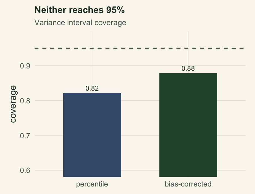
The percentile interval covers 82% of the time and the bias-corrected interval 88%, both short of 95%. The correction helps, as it did for the skewed ratio in the first post, but it is not a guarantee, and at this sample size neither reaches the promised level. The point is not which interval wins; it is that the nominal level is optimistic and you cannot know by how much without checking. When you can simulate, as we have throughout, do it and read the actual coverage. When you cannot, prefer the bias-corrected interval, report the resampling scheme and the number of resamples, and treat 95% as a hopeful label. For an automatic correction, the double bootstrap re-calibrates the nominal level using an inner resample, at a squared cost in computation.

Figure 3: Coverage of the plain percentile and the bias-corrected 95% intervals for a variance over many samples. Both fall short of nominal; the correction narrows the gap but does not close it.

What to take away

Resampling is a tool, not a guarantee, and this series has tried to show both its reach and its edges. It rescues honest uncertainty from awkward statistics like a ratio, it builds null distributions that asymptotics get wrong, and it adapts to dependence through blocks and clusters. But it needs a smooth statistic, enough data to resolve it, and the right resampling unit; and even then its intervals lean a little narrow. The habit that ties the series together is to check rather than assume: inspect the bootstrap distribution, ask whether the statistic is smooth and the observations are independent, and verify coverage by simulation whenever you can. A bootstrap you have checked is a strong instrument. A bootstrap you have merely run is a guess with decimals.

Related tutorials

• The nonparametric bootstrap
• The parametric bootstrap
• Bootstrapping dependent data
• Checking a nonlinear model

References

Bickel and Freedman 1981 Annals of Statistics 9(6):1196-1217 (10.1214/aos/1176345637)

Andrews 2000 Econometrica 68(2):399-405 (10.1111/1468-0262.00114)

Canty, Davison, Hinkley and Ventura 2006 Canadian Journal of Statistics 34(1):5-27 (10.1002/cjs.5550340103)

Puth, Neuhauser and Ruxton 2015 Journal of Animal Ecology 84(4):892-897 (10.1111/1365-2656.12382)

Davison and Hinkley 1997 Bootstrap Methods and their Application. ISBN 978-0-521-57391-7