set.seed(34)
mlc <- log(26); slc <- 0.62          # control: meanlog, sdlog
mli <- log(52); sli <- 0.78          # impact: larger and more variable
rr_true <- exp(mli + sli^2/2) / exp(mlc + slc^2/2)   # ratio of population means

nc <- 20; ni <- 22
xc <- rlnorm(nc, mlc, slc)           # control abundances
xi <- rlnorm(ni, mli, sli)           # impact abundances
resp_ratio <- function(a, b) mean(b) / mean(a)
theta_hat <- resp_ratio(xc, xi)
The nonparametric bootstrap from scratch
R
resampling
statistics
ecology tutorial
Resample your data to approximate a sampling distribution, and build percentile, basic and BCa intervals by hand for a skewed ecological response ratio.
Corrected 7 October 2026: the coverage section said BCa comes closest to the target split of misses below and above the truth; it now says BCa comes closest to an even split, since the percentile interval is closer to the target on each side. The interval section said the BCa correction pushes the interval into the tail where the real uncertainty lives; it now says BCa sets both limits higher than the percentile interval does and leaves it to the coverage check whether that helps.
Corrected 30 September 2026: the post said BCa splits the risk of missing correctly and that this is the real reason to prefer it; it now says BCa spreads its misses most evenly but still misses too often on each side, and that the percentile interval comes closer to the target in this simulation. The take-away also said BCa is worth its extra width; it now says that in the simulation BCa was a little wider than the percentile interval and still covered less often.
Many quantities an ecologist reports have no textbook standard error. A response ratio, a coefficient of variation, a diversity index, a ratio of slopes: each is a smooth function of the data, but the formula for its uncertainty is either ugly or unknown. The bootstrap sidesteps that. It treats the sample as a stand-in for the population and asks a mechanical question: if I could redraw the data many times, how much would my estimate move? We answer it by redrawing from the data we already have.
This post builds the nonparametric bootstrap by hand for a response ratio, the ratio of two group means that turns up constantly in impact studies and meta-analysis. We compute a bootstrap standard error, then three flavours of confidence interval (percentile, basic and bias-corrected-and-accelerated), and finish by checking which one actually covers the truth. The recurring lesson of this series starts here: a resampled interval is only as honest as the assumptions behind the flavour you picked.
The idea in one paragraph
Write the estimator as a function of the sample, theta_hat = t(x). Its sampling distribution (how theta_hat would vary across repeated samples from the population) is what we cannot see, because we have one sample. The bootstrap replaces the unknown population with the empirical distribution: draw a resample of the same size with replacement from the observed data, recompute the statistic, and repeat many times. The spread of those resampled statistics estimates the spread of the real sampling distribution. Nothing about the estimator needs to be linear or normal.
A response ratio with a skewed sampling distribution
Abundance data are typically right-skewed, so we simulate control and impact counts from lognormal distributions and take the ratio of their means. The true ratio is fixed by the population means, so we can judge every interval against it later.
The two samples give control and impact means of 29.5 and 67.3, so the observed response ratio is 2.286 against a true value of 2.237. A single sample can land some way from the truth; that is exactly why we want an interval rather than a point.
Resampling by hand
Each bootstrap replicate resamples within each group with replacement, keeping the two sample sizes fixed, and recomputes the ratio. The standard error is just the standard deviation of those replicates.
set.seed(101)
B <- 4000
boot <- replicate(B, mean(sample(xi, ni, replace = TRUE)) /
                     mean(sample(xc, nc, replace = TRUE)))
se_boot   <- sd(boot)
bias_boot <- mean(boot) - theta_hat
skew_boot <- mean((boot - mean(boot))^3) / sd(boot)^3
The bootstrap standard error is 0.599, and the bootstrap distribution is distinctly right-skewed (skewness 0.76). That skew is the whole reason the interval flavours will disagree: a ratio of positive quantities has a longer upper tail, and any method that forces symmetry will get the shape wrong.
Four intervals, four shapes
The normal interval takes theta_hat plus or minus 1.96 bootstrap standard errors, so it is symmetric by construction. The percentile interval reads the 2.5th and 97.5th percentiles straight off the bootstrap distribution, inheriting its skew. The basic (reverse-percentile) interval reflects those percentiles through the estimate. The BCa interval adjusts the percentiles for two things a bare percentile ignores: median bias (through z0, the fraction of replicates below the estimate, mapped to a normal score) and how fast the standard error changes with the parameter (the acceleration a, from the jackknife skewness).
ci_norm  <- theta_hat + c(-1, 1) * qnorm(0.975) * se_boot
ci_perc  <- as.numeric(quantile(boot, c(0.025, 0.975)))
ci_basic <- as.numeric(2 * theta_hat - quantile(boot, c(0.975, 0.025)))

# BCa: bias-correction z0 and acceleration a (jackknife)
z0   <- qnorm(mean(boot < theta_hat))
jack <- c(sapply(seq_len(nc), function(i) resp_ratio(xc[-i], xi)),
          sapply(seq_len(ni), function(i) resp_ratio(xc, xi[-i])))
jbar <- mean(jack)
acc  <- sum((jbar - jack)^3) / (6 * (sum((jbar - jack)^2))^1.5)
zc   <- qnorm(c(0.025, 0.975))
adj  <- pnorm(z0 + (z0 + zc) / (1 - acc * (z0 + zc)))
ci_bca <- as.numeric(quantile(boot, adj))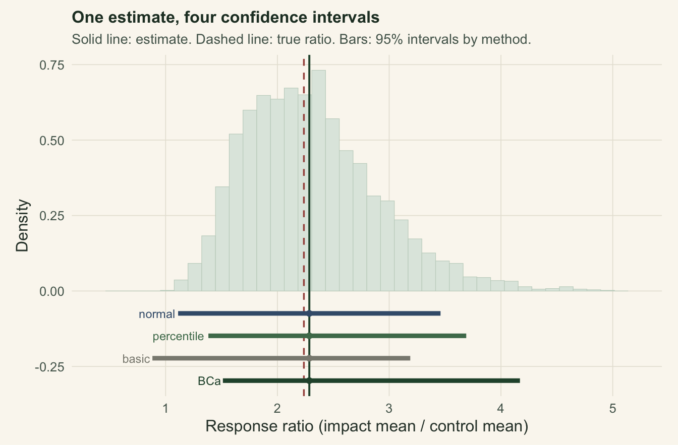
The normal interval runs 1.11 to 3.46, with equal arms of 1.17 on each side. The BCa interval runs 1.51 to 4.17, with a short lower arm of 0.77 and a long upper arm of 1.88. The bias correction here is mild (z0 is 0.071, acceleration 0.082), yet it still sets both limits higher than the percentile interval does, pushing the interval further into the upper tail; the coverage check below asks whether that helps. The basic interval reflects the skew the other way, which is a warning sign: reflecting a skewed distribution can send the interval away from where the mass actually is.
Which interval covers the truth?
Shapes are suggestive; coverage is the test. We know the true ratio, so we can redraw the whole study many times, build each interval on each dataset, and count how often it traps the truth. A 95% interval should succeed 95% of the time.
covsim <- function(R = 1500, Bb = 800) {
  hit <- matrix(0, R, 4); mlo <- matrix(0, R, 4); mhi <- matrix(0, R, 4)
  for (r in seq_len(R)) {
    a <- rlnorm(nc, mlc, slc); b <- rlnorm(ni, mli, sli)
    th <- resp_ratio(a, b)
    bt <- replicate(Bb, mean(sample(b, ni, TRUE)) / mean(sample(a, nc, TRUE)))
    se <- sd(bt)
    c_n <- th + c(-1, 1) * qnorm(0.975) * se
    c_p <- quantile(bt, c(0.025, 0.975))
    c_b <- 2 * th - quantile(bt, c(0.975, 0.025))
    z0b <- qnorm(mean(bt < th))
    jk  <- c(sapply(seq_len(nc), function(i) resp_ratio(a[-i], b)),
             sapply(seq_len(ni), function(i) resp_ratio(a, b[-i])))
    jbb <- mean(jk); ac <- sum((jbb - jk)^3) / (6 * (sum((jbb - jk)^2))^1.5)
    ad  <- pnorm(z0b + (z0b + zc) / (1 - ac * (z0b + zc)))
    c_c <- quantile(bt, ad)
    L <- list(c_n, as.numeric(c_p), as.numeric(c_b), as.numeric(c_c))
    for (k in 1:4) {
      hit[r, k] <- (rr_true >= L[[k]][1] & rr_true <= L[[k]][2])
      mlo[r, k] <- (rr_true <  L[[k]][1])          # missed below
      mhi[r, k] <- (rr_true >  L[[k]][2])          # missed above
    }
  }
  list(cov = colMeans(hit), miss_lo = colMeans(mlo), miss_hi = colMeans(mhi))
}
set.seed(202)
cvr <- covsim(R = 1500, Bb = 800)
cov_norm <- cvr$cov[1]; cov_perc <- cvr$cov[2]; cov_basic <- cvr$cov[3]; cov_bca <- cvr$cov[4]
hi_norm <- cvr$miss_hi[1]; lo_norm <- cvr$miss_lo[1]
hi_basic <- cvr$miss_hi[3]; lo_basic <- cvr$miss_lo[3]
lo_bca <- cvr$miss_lo[4]; hi_bca <- cvr$miss_hi[4]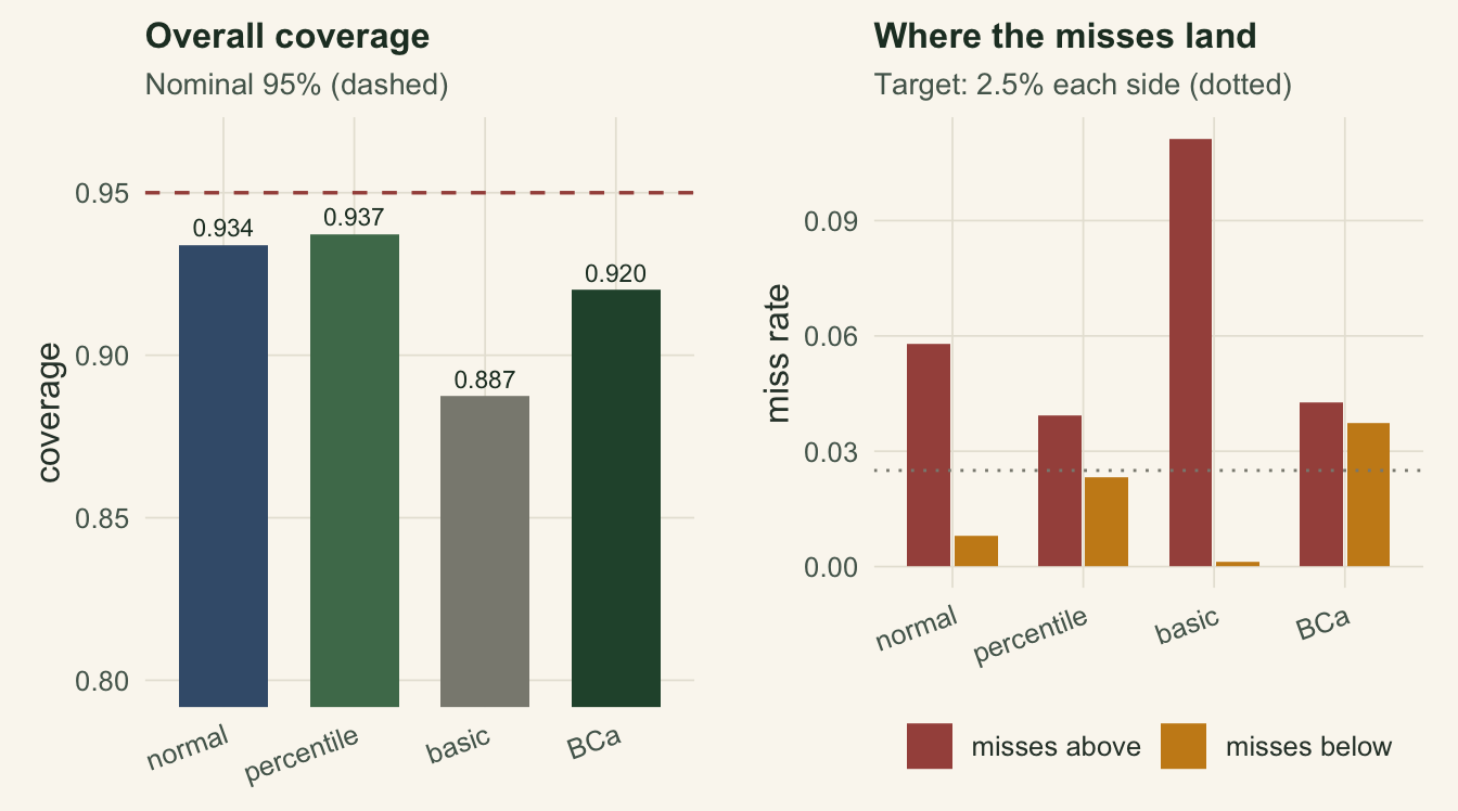
Every method falls short of 95%: percentile reaches 93.7%, normal 93.4%, BCa 92.0%, and the reflected basic interval is clearly worst at 88.7%. But the overall number hides the more telling failure, which is where each interval misses. A calibrated 95% interval should miss about 2.5% above the truth and 2.5% below. BCa comes closest to an even split, missing 3.7% low and 4.3% high. The symmetric normal interval misses high 5.8% of the time against only 0.8% low, and the basic interval is worse still, with almost all of its 11.3% failures (11.1% high versus 0.1% low) on the high side. Both sit too far left because they refuse to lean into the right skew. That imbalance matters more than the headline coverage. BCa spreads its misses most evenly, although it still misses more than 2.5% on each side; in this simulation the percentile interval, missing 2.3% low and 3.9% high, comes closer to the target on both sides.
What to take away
The nonparametric bootstrap is close to free: a few lines of resampling give you a standard error and an interval for an estimator that has no clean formula. The price is that the interval is an approximation whose accuracy depends on the flavour. For a skewed statistic, a symmetric normal interval mislabels the shape and the basic interval can reflect the skew the wrong way. BCa corrects for bias and for how the spread changes with the parameter, and it spread its misses most evenly, but in the simulation above it was on average a little wider than the percentile interval and still covered less often. Whichever you use, remember that the nominal coverage is optimistic, and always say which interval you computed and how many resamples you used. The next post keeps the resampling idea but changes what we resample from: instead of the data, we resample from a fitted model.
References
Efron 1979 Annals of Statistics 7(1):1-26 (10.1214/aos/1176344552)
Efron 1987 Journal of the American Statistical Association 82(397):171-185 (10.1080/01621459.1987.10478410)
DiCiccio and Efron 1996 Statistical Science 11(3):189-228 (10.1214/ss/1032280214)
Puth, Neuhauser and Ruxton 2015 Journal of Animal Ecology 84(4):892-897 (10.1111/1365-2656.12382)
Efron and Tibshirani 1993 An Introduction to the Bootstrap. ISBN 978-0-412-04231-7