library(ggplot2)
te <- c(forest = "#2f5d50", moss = "#7a9b76", rust = "#b5651d", gold = "#c9a227",
        slate = "#3d4b53", sand = "#d9cbb2", sky = "#5b8aa6", brick = "#8c3b2e")
theme_te <- function(base_size = 12) {
  theme_minimal(base_size = base_size) +
    theme(panel.grid.minor = element_blank(),
          panel.grid.major = element_line(colour = "#e7e1d5", linewidth = 0.3),
          axis.title = element_text(colour = "#3d4b53"),
          axis.text  = element_text(colour = "#5c6670"),
          plot.title = element_text(colour = "#2f3a40", face = "bold", size = base_size + 1),
          plot.subtitle = element_text(colour = "#5c6670", size = base_size - 1),
          legend.position = "bottom",
          legend.title = element_text(colour = "#3d4b53"),
          plot.background  = element_rect(fill = "#f5f4ee", colour = NA),
          panel.background = element_rect(fill = "#f5f4ee", colour = NA))
}
covCJ <- function(x) { n <- sum(x); f1 <- sum(x == 1); f2 <- sum(x == 2)
  if (f2 == 0) f2 <- f1 * (f1 - 1) / 2
  1 - (f1 / n) * ((n - 1) * f1 / ((n - 1) * f1 + 2 * f2)) }
chao1 <- function(x) { n <- sum(x); f1 <- sum(x == 1); f2 <- sum(x == 2)
length(x) + (n - 1) / n * f1 * (f1 - 1) / (2 * (f2 + 1)) }Checking a diversity estimate
R
species richness
model diagnostics
ecology tutorial
A richness estimate is only as sound as its rarest counts. Check coverage, singleton sensitivity, interval coverage and how much of a finite frame you sampled.
Updated 27 September 2026: a new section, Check four: how much of the frame did you sample?, measures on the complete Barro Colorado Island tree census how far Chao2 overshoots the known richness of a finite set of quadrats as a larger share of them is sampled, and how the without-replacement bound of Chao and Lin (2012) compares.
Corrected 25 September 2026: the coverage check said the coverage deficit is roughly how much of the estimate is projection. The deficit is the chance that the next individual belongs to a species not yet recorded; the share of the estimate that is projection is larger, and the passage now prints both.
The earlier posts in this cluster produced richness and diversity estimates that beat the naive observed counts. This one turns them over and asks how far to trust them. The theme running through the whole cluster is that the unseen species are not recoverable from the seen without an assumption, so the honest question is not “what is the estimate” but “what does the estimate depend on, and how much”. Three checks answer that: how far you are extrapolating, how much the estimate rides on a fragile count, and whether its confidence interval means what it seems to. A fourth asks whether the units you sampled are most of a finite set, which changes what the estimate is an estimate of.
set.seed(4193)
S_true <- 180
rel <- exp(rnorm(S_true, 0, 1.6)); rel <- rel / sum(rel)
Check one: how far are you extrapolating?
Sample coverage is the plainest reliability check. It estimates what fraction of the community’s individuals belong to species you have already seen, so the deficit, one minus coverage, estimates the chance that the next individual belongs to a species not yet recorded. It is not the share of species still missing, nor the share of the estimate that is projection: on this community both are larger, because the missing species are rare (Coverage-based rarefaction and extrapolation measures the gap on the same community). Compare a light effort with a heavy one on the same community.
n_low <- 250; n_high <- 1500
x_lo <- as.vector(rmultinom(1, n_low,  rel)); x_lo <- x_lo[x_lo > 0]
x_hi <- as.vector(rmultinom(1, n_high, rel)); x_hi <- x_hi[x_hi > 0]
data.frame(effort = c("low (n = 250)", "high (n = 1500)"),
           S_obs   = c(length(x_lo), length(x_hi)),
           coverage = round(c(covCJ(x_lo), covCJ(x_hi)), 4),
           Chao1    = round(c(chao1(x_lo), chao1(x_hi)), 1),
           unseen   = round(c(chao1(x_lo) - length(x_lo), chao1(x_hi) - length(x_hi)), 1))
effort S_obs coverage Chao1 unseen
1 low (n = 250) 73 0.8764 103.9 30.9
2 high (n = 1500) 134 0.9834 147.0 13.0The light sample reaches 0.876 coverage and asks Chao1 to invent 30.9 unseen species on top of the 73 observed: 30 per cent of the estimate, against a coverage deficit of 12 per cent, while 59 per cent of the 180 species are in truth still unseen. The heavy sample reaches 0.983 coverage, so its estimate leans on only 13 projected species (9 per cent of it, against a deficit of 2 per cent) and sits much closer to the true 180. Low coverage is a warning that much of the estimate is extrapolation, and extrapolation is where assumptions do the work.
Check two: does the estimate ride on the singletons?
Chao1 is built from singletons and doubletons, so the singleton count is load-bearing. That matters because singletons are exactly the counts most easily corrupted: a misidentification, a contaminant, a sequencing error in a metabarcoding run all masquerade as a species seen once. Vary the singleton count and watch the estimate move.
x <- x_lo; So <- length(x); f1 <- sum(x == 1); f2 <- sum(x == 2); nn <- sum(x)
chao1_f1 <- function(f1v) So + (nn - 1) / nn * f1v * (f1v - 1) / (2 * (f2 + 1))
c(f1_observed = f1, f2 = f2,
  Chao1_observed = round(chao1_f1(f1), 1),
  Chao1_if_20pct_spurious = round(chao1_f1(round(f1 * 0.8)), 1),
  Chao1_if_20pct_more     = round(chao1_f1(round(f1 * 1.2)), 1),
  slope_per_singleton = round(chao1_f1(f1 + 1) - chao1_f1(f1), 2))
f1_observed f2 Chao1_observed
31.00 14.00 103.90
Chao1_if_20pct_spurious Chao1_if_20pct_more slope_per_singleton
92.90 117.20 2.06 With 31 singletons the estimate is 103.9. Treat a fifth of them as spurious and it drops to 92.9; add a fifth and it climbs to 117.2. Near the observed value each singleton is worth about 2.06 species of estimated richness. An estimate this sensitive to a fragile count deserves a hard look at where the singletons came from; corrected estimators that down-weight spurious singletons exist for exactly this reason.
f1grid <- seq(max(2, round(f1 * 0.6)), round(f1 * 1.4), by = 1)
fb <- data.frame(f1 = f1grid, chao1 = sapply(f1grid, chao1_f1))
marks <- data.frame(f1 = c(round(f1 * 0.8), f1, round(f1 * 1.2)),
                    chao1 = chao1_f1(c(round(f1 * 0.8), f1, round(f1 * 1.2))))
p_singleton <- ggplot(fb, aes(f1, chao1)) +
  geom_line(colour = te["forest"], linewidth = 0.9) +
  geom_point(data = marks, colour = te["rust"], size = 3) +
  geom_text(data = marks, aes(label = round(chao1)), vjust = -1.1, size = 3, colour = te["slate"]) +
  labs(title = "Chao1 rides on the singleton count",
       subtitle = "A 20% change in singletons (miscounts, contamination) moves the estimate by about 12 species",
       x = "number of singletons (species seen once)", y = "Chao1 richness estimate") +
  theme_te()
p_singleton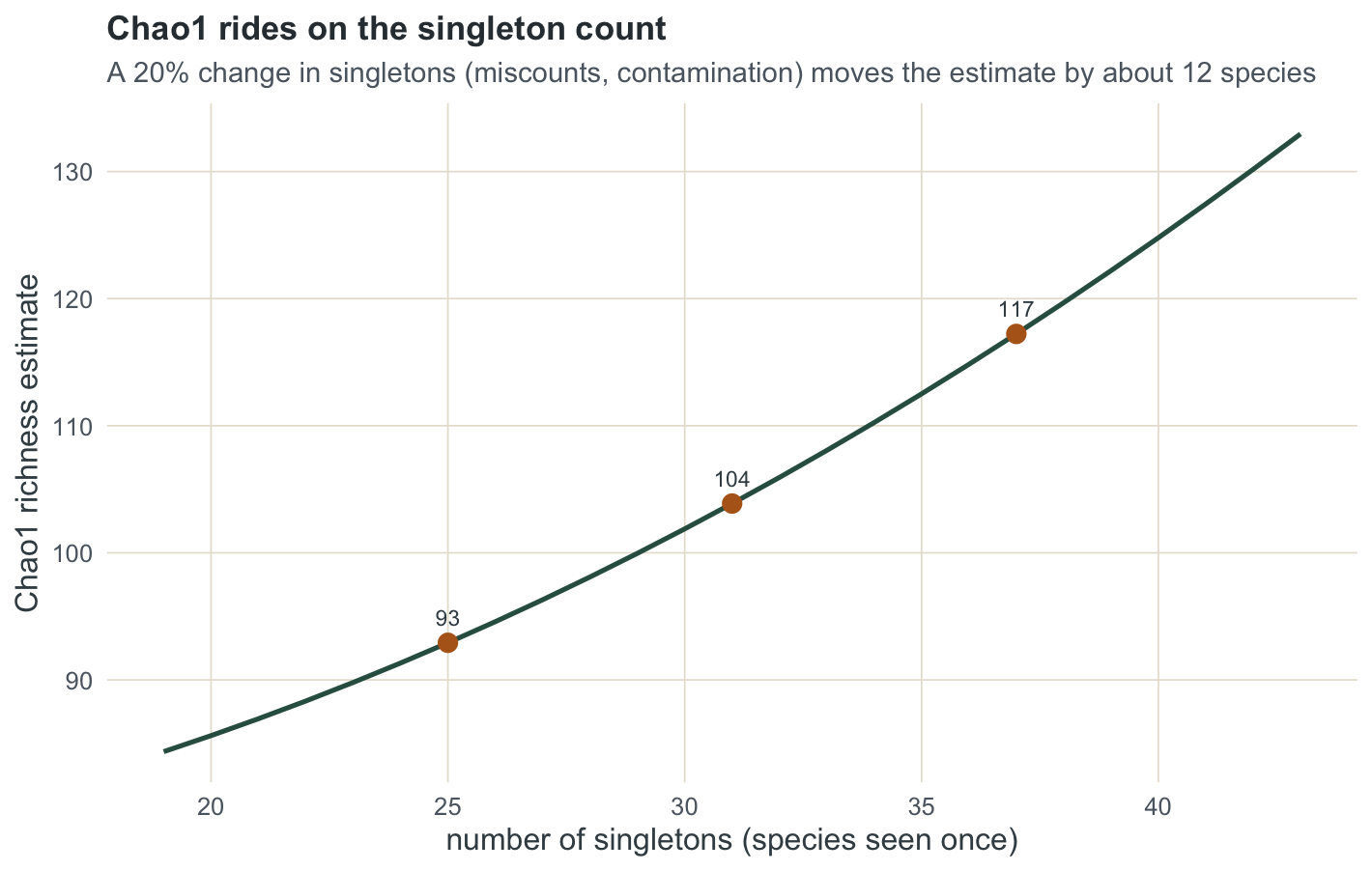
Check three: what does the confidence interval cover?
Chao’s variance formula gives an interval, but the symmetric version misbehaves because the estimator’s sampling distribution is right-skewed. The log-transformed interval fixes the shape and keeps the lower limit above the observed richness. One mismatch is worth naming first. The variance below is Chao’s original formula for the uncorrected estimator S_obs + f1^2/(2 f2), which on these counts gives 107.3 species, while the point estimate it is wrapped around is the bias-corrected 103.9. The interval is centred on one estimator and scaled by the variance of another, which is exactly the sort of unstated mismatch this post is about. The deeper point is what either interval is an interval for.
chao1_ci <- function(x, level = 0.95) { n <- sum(x); So <- length(x)
  f1 <- sum(x == 1); f2 <- sum(x == 2); Sc <- chao1(x); D <- Sc - So
  r <- f1 / f2; v <- f2 * (0.5 * r^2 + r^3 + 0.25 * r^4)     # Chao 1987 variance
  z <- qnorm(1 - (1 - level) / 2)
  wald <- c(Sc - z * sqrt(v), Sc + z * sqrt(v))
  K <- exp(z * sqrt(log(1 + v / D^2)))                        # log-transformed
  list(Sc = Sc, wald = wald, logci = c(So + D / K, So + D * K)) }
ci <- chao1_ci(x_lo)
c(Chao1 = round(ci$Sc, 1), Chao1_uncorrected = round(So + f1^2 / (2 * f2), 1),
  Wald_lo = round(ci$wald[1], 1), Wald_hi = round(ci$wald[2], 1),
  log_lo = round(ci$logci[1], 1), log_hi = round(ci$logci[2], 1))
Chao1 Chao1_uncorrected Wald_lo Wald_hi
103.9 107.3 71.6 136.1
log_lo log_hi
84.6 155.2 Now check both intervals by simulation, against two targets: the estimator’s own expectation, and the true richness.
set.seed(5193); R <- 2000
Sc <- wl <- wh <- ll <- lh <- numeric(R)
for (r in 1:R) { xx <- as.vector(rmultinom(1, n_low, rel)); xx <- xx[xx > 0]
  ci <- chao1_ci(xx); Sc[r] <- ci$Sc
  wl[r] <- ci$wald[1]; wh[r] <- ci$wald[2]; ll[r] <- ci$logci[1]; lh[r] <- ci$logci[2] }
E_chao1 <- mean(Sc)
data.frame(target = c("E[Chao1] (estimator)", "true richness"),
  Wald = round(c(mean(wl <= E_chao1 & wh >= E_chao1), mean(wl <= S_true & wh >= S_true)), 3),
  log  = round(c(mean(ll <= E_chao1 & lh >= E_chao1), mean(ll <= S_true & lh >= S_true)), 3))
target Wald log
1 E[Chao1] (estimator) 0.899 0.962
2 true richness 0.230 0.427fc <- data.frame(
method = factor(rep(c("symmetric Wald", "log-transformed"), each = 2),
levels = c("symmetric Wald", "log-transformed")),
target = rep(c("E[Chao1] (estimator target)", "true richness"), 2),
coverage = c(mean(wl <= E_chao1 & wh >= E_chao1), mean(wl <= S_true & wh >= S_true),
mean(ll <= E_chao1 & lh >= E_chao1), mean(ll <= S_true & lh >= S_true)))
ggplot(fc, aes(method, coverage, fill = target)) +
geom_hline(yintercept = 0.95, linetype = "dashed", colour = te["brick"], linewidth = 0.5) +
geom_col(position = position_dodge(width = 0.7), width = 0.6) +
geom_text(aes(label = sprintf("%.2f", coverage)), position = position_dodge(width = 0.7),
vjust = -0.4, size = 3, colour = te["slate"]) +
scale_fill_manual(values = c("E[Chao1] (estimator target)" = unname(te["forest"]),
"true richness" = unname(te["sky"])), name = NULL) +
scale_y_continuous(limits = c(0, 1.05)) +
labs(title = "The interval covers the lower bound, not the truth",
subtitle = paste0("n = 250, 2000 samples; dashed line 0.95:\n",
"log CI reaches the estimator target, neither reaches true richness 180"),
x = NULL, y = "interval coverage") +
theme_te()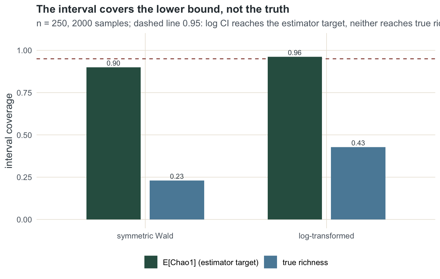
The mean Chao1 across samples is 116.8, and the log-transformed interval covers that at about 0.96, close to the nominal 0.95, while the symmetric interval falls to 0.9. So the log interval is the right construction. But watch the second target: neither interval covers the true richness of 180, at 0.23 and 0.43. That is not a broken interval. It is Chao1 being a lower bound: the interval brackets the estimator, and the estimator sits below the truth by construction.
Check four: how much of the frame did you sample?
The three checks above assume a community with no edge: there is always another individual, or another quadrat, to sample. Many surveys instead cover a fixed and finite set of units, the ponds of one catchment, the islands of an archipelago, the cells of a reserve grid, and when a large share of them has been surveyed the richness of that set is the natural target. Chao and Lin (2012) showed that estimators built for sampling with replacement overshoot such a target at high sampling fractions and do not converge to it as the fraction approaches one, and they derived a lower bound for sampling without replacement. This check reproduces their result on real data where the answer is known. The BCI data in vegan count every tree of at least 10 cm diameter at breast height in each of 50 one-hectare quadrats that tile the Barro Colorado Island plot (Condit et al. 2002), so the richness of that frame (those quadrats, that size class, that census) is not an estimate: it is the number of columns.
Draw k of the 50 quadrats without replacement, a sampling fraction q = k / 50, and compare three numbers with the census: the species observed; Chao2, the incidence version of Chao1 from Estimating species richness beyond your sample, in its classic form S_obs + (k - 1) / k * Q1^2 / (2 Q2) (Chao and Colwell 2017, eq. 2b), where Q1 and Q2 count the species found in exactly one and exactly two of the sampled quadrats; and the without-replacement bound S_obs + Q1^2 / (2 w Q2 + r Q1) with w = k / (k - 1) and r equal to q / (1 - q) (their eq. 9c). As q goes to zero the bound becomes the classic Chao2, which is why the classic form, not the bias-corrected one in the chao1() helper above, is the fair comparison.
data("BCI", package = "vegan")          # the data set only; vegan is not attached
stopifnot(identical(dim(BCI), c(50L, 225L)), sum(BCI) == 21457, all(colSums(BCI) > 0))
bci_inc <- (BCI > 0) * 1; bci_K <- nrow(bci_inc); bci_S <- ncol(bci_inc)   # incidence
bci_est <- function(y, K) { k <- nrow(y); qq <- colSums(y); qq <- qq[qq > 0]
  S <- length(qq); Q1 <- sum(qq == 1); Q2 <- sum(qq == 2); q <- k / K
  c(S_obs = S, Q2 = Q2, chao2 = S + (k - 1) / k * Q1^2 / (2 * Q2),
    wor = if (q < 1) S + Q1^2 / (2 * k / (k - 1) * Q2 + q / (1 - q) * Q1) else S) }
set.seed(27092601); bci_q <- c(0.2, 0.3, 0.4, 0.5, 0.7, 0.9); bci_reps <- 300
bci_draws <- lapply(bci_q, function(q) t(replicate(bci_reps,
  bci_est(bci_inc[sample.int(bci_K, round(q * bci_K)), ], bci_K))))
stopifnot(all(sapply(bci_draws, function(m) min(m[, "Q2"])) > 0))
bci_col <- function(v, f) sapply(bci_draws, function(m) f(m[, v]))
bci_tab <- data.frame(q = bci_q, k = round(bci_q * bci_K),
  err_S_obs = bci_col("S_obs", mean) - bci_S, err_chao2 = bci_col("chao2", mean) - bci_S,
  err_wor = bci_col("wor", mean) - bci_S, chao2_over = bci_col("chao2", function(v) mean(v > bci_S)),
  wor_over = bci_col("wor", function(v) mean(v > bci_S)))
bci_mcse <- max(bci_col("chao2", sd), bci_col("wor", sd)) / sqrt(bci_reps)
bci_at <- function(q) bci_tab[abs(bci_tab$q - q) < 1e-9, ]
bci_whole <- bci_est(bci_inc, Inf)       # the frame read as a sample from an unlimited supply
bci_Q1 <- sum(colSums(bci_inc) == 1); bci_Q2 <- sum(colSums(bci_inc) == 2)
bci_over <- (bci_K - 1) / bci_K * bci_Q1^2 / (2 * bci_Q2)
bci_single <- sum(colSums(BCI) == 1)     # species with one tree in the whole census
stopifnot(abs(bci_whole[["chao2"]] - bci_S - bci_over) < 1e-9,
          abs(vegan::specpool(BCI)$chao - bci_whole[["chao2"]]) < 1e-9)
round(bci_tab, 2)
q k err_S_obs err_chao2 err_wor chao2_over wor_over
1 0.2 10 -42.60 -20.14 -23.63 0.06 0.01
2 0.3 15 -30.18 -4.77 -11.93 0.30 0.08
3 0.4 20 -22.38 3.55 -6.62 0.59 0.17
4 0.5 25 -17.02 8.51 -4.24 0.73 0.26
5 0.7 35 -8.19 12.30 -1.27 0.91 0.36
6 0.9 45 -2.28 12.26 -0.15 0.99 0.52bci_long <- do.call(rbind, lapply(seq_along(bci_q), function(i)
do.call(rbind, lapply(c("S_obs", "chao2", "wor"), function(v) { vv <- bci_draws[[i]][, v]
data.frame(q = bci_q[i], what = v, mean = mean(vv), lo = quantile(vv, 0.1, names = FALSE),
hi = quantile(vv, 0.9, names = FALSE)) }))))
bci_long$what <- factor(bci_long$what, levels = c("S_obs", "chao2", "wor"),
labels = c("species observed", "Chao2 (assumes replacement)", "bound without replacement"))
bci_cols <- setNames(unname(te[c("slate", "rust", "forest")]), levels(bci_long$what))
ggplot(bci_long, aes(q, mean, colour = what, fill = what)) +
geom_hline(yintercept = bci_S, linetype = "dashed", colour = te["brick"], linewidth = 0.5) +
geom_ribbon(data = bci_long[bci_long$what != "species observed", ],
aes(ymin = lo, ymax = hi), alpha = 0.15, colour = NA) +
geom_line(linewidth = 0.9) + geom_point(size = 2) +
annotate("point", x = 1, y = bci_whole[["chao2"]], shape = 21, size = 3, stroke = 1,
colour = te["rust"], fill = "#f5f4ee") +
annotate("text", x = 0.2, y = bci_S + 3, label = paste("census richness", bci_S), hjust = 0,
size = 3, colour = te["brick"]) +
scale_colour_manual(values = bci_cols, name = NULL, aesthetics = c("colour", "fill")) +
scale_x_continuous(breaks = c(bci_q, 1)) +
labs(title = "On a finite frame Chao2 overshoots as the sampled share grows",
subtitle = "BCI, 50 one-hectare quadrats drawn without replacement, 300 draws per share",
x = "share of the quadrats sampled (q = k / 50)", y = "richness") +
guides(fill = "none") + theme_te()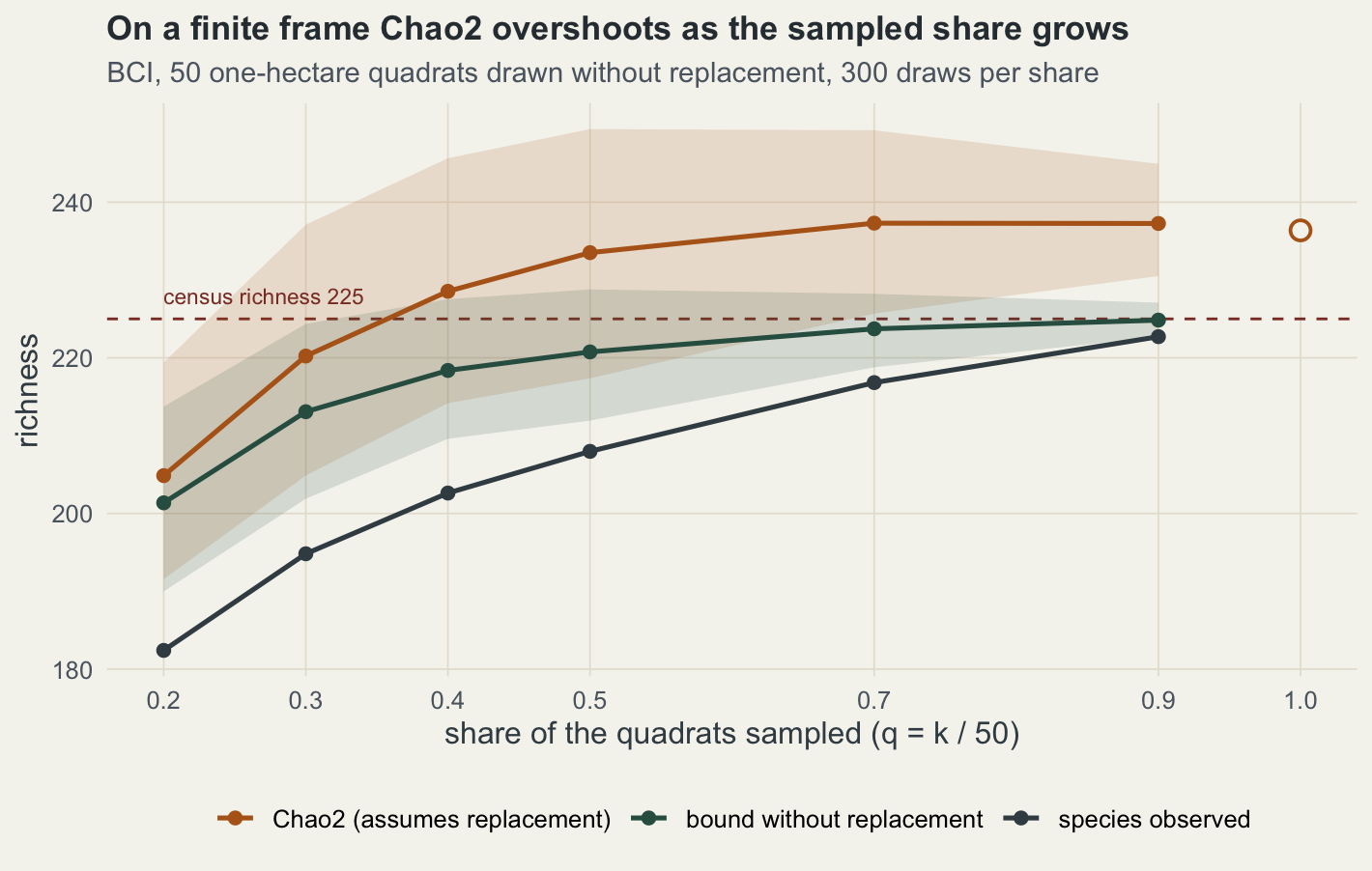
With half the quadrats in hand (q = 0.5) Chao2 lands on average 8.5 species above the census richness of 225, and the without-replacement bound 4.2 below it; with 45 of the 50 quadrats (q = 0.9) Chao2 is 12.3 above and the bound 0.2 below. Chao2’s mean error changes sign between q = 0.3 (-4.8) and 0.4 (+3.5), and at q = 0.9 it exceeds the census in 0.99 of the draws. Monte Carlo standard errors of these means are at most 0.8. The overshoot at the top end is closed form: with every quadrat in hand the observed richness is the census, and Chao2 still adds (k - 1) / k * Q1^2 / (2 Q2) at k = 50, which with 21 uniques and 19 duplicates among the 50 quadrats is 11.4 species, for a total of 236.4; vegan::specpool() returns the same value (the chunk stops if it does not).
That 236.4 is not a wrong answer to its own question. Read as a sample, the 50 quadrats stand for an unlimited supply of one-hectare quadrats like them, and Chao2 estimates a lower bound for the richness of that larger set, which is a different quantity from the richness of these 50. Even the complete census holds 19 species represented by a single tree, a reminder that 225 is the richness of this frame, not of the forest around it.
The bound is not free. At q = 0.2 and 0.3 it lies further below the census than Chao2 does (-23.6 against -20.1, -11.9 against -4.8), its mean miss is the smaller of the two only from q = 0.5 on, and it is a lower bound in the mean only: at q = 0.9 it exceeds the census in 0.52 of the draws. Both the overshoot and the repair are Chao and Lin’s result, and they tested it on subsamples of real censuses too; BCI lets you watch it with a data set that ships with vegan. For your own data the check is a question about the frame. If the units you surveyed are most of a finite set and the richness of that set is what you report, state the sampling fraction and use the without-replacement form; if the units stand for a wider landscape, Chao2 is aimed at that wider target instead.
What the number can promise
Read the four checks together and the estimate stops being a single figure and becomes a claim with conditions attached. It is a lower bound for the community the units were drawn from (and can overshoot the richness of a finite set whose units are mostly in hand), its interval is a confidence statement about that lower bound, and both depend on sample coverage and on a singleton count that field or laboratory error can distort. This is the same shape as the honest limits elsewhere on the blog: the discovery set that depends on the chosen error rate, the effect whose sign depends on an unmeasured reference frame. The estimate is a function of what you assume about the unseen, not a fact about the community, and the checks make the assumptions visible rather than pretending they are not there.
References
Chao A 1987 Biometrics 43(4):783-791 (10.2307/2531532)
Colwell R K, Chao A, Gotelli N J, Lin S-Y, Mao C X, Chazdon R L, Longino J T 2012 Journal of Plant Ecology 5(1):3-21 (10.1093/jpe/rtr044)
Chao A, Jost L 2012 Ecology 93(12):2533-2547 (10.1890/11-1952.1)
Walther B A, Moore J L 2005 Ecography 28(6):815-829 (10.1111/j.2005.0906-7590.04112.x)
Chiu C-H, Chao A 2016 PeerJ 4:e1634 (10.7717/peerj.1634)
Chao A, Lin C-W 2012 Biometrics 68(3):912-921 (10.1111/j.1541-0420.2011.01739.x)
Chao A, Colwell R K 2017 SORT (Statistics and Operations Research Transactions) 41(1):3-54 (10.2436/20.8080.02.49)
Condit R, Pitman N, Leigh E G Jr, Chave J, Terborgh J, Foster R B, Nunez P, Aguilar S, Valencia R, Villa G, Muller-Landau H C, Losos E, Hubbell S P 2002 Science 295(5555):666-669 (10.1126/science.1066854)