library(ggplot2); library(dplyr); library(tidyr)
te <- c(forest = "#2f5d50", moss = "#7a9b76", rust = "#b5651d", gold = "#c9a227",
        slate = "#3d4b53", sand = "#d9cbb2", sky = "#5b8aa6", brick = "#8c3b2e")
theme_te <- function(base_size = 12) {
  theme_minimal(base_size = base_size) +
    theme(panel.grid.minor = element_blank(),
          panel.grid.major = element_line(colour = "#e7e1d5", linewidth = 0.3),
          axis.title = element_text(colour = "#3d4b53"),
          axis.text  = element_text(colour = "#5c6670"),
          plot.title = element_text(colour = "#2f3a40", face = "bold", size = base_size + 1),
          plot.subtitle = element_text(colour = "#5c6670", size = base_size - 1),
          legend.position = "bottom",
          legend.title = element_text(colour = "#3d4b53"),
          plot.background  = element_rect(fill = "#f5f4ee", colour = NA),
          panel.background = element_rect(fill = "#f5f4ee", colour = NA))
}Estimating species richness beyond your sample
R
species richness
biodiversity
ecology tutorial
Observed species counts undersample true richness. Estimate the unseen with Chao1, ACE and jackknife estimators in base R, and see why they stay lower bounds.
Step 14 of the Tidy Ecology course, Part three: describe the community.
Count the species in a plot, a light trap or a metabarcoding run and you have a number. It is almost never the number you want. Rare species slip through, and the ones you never saw contribute nothing to the tally, so the observed richness S_obs is a downward-biased estimate of how many species are actually there. This post builds the standard non-parametric richness estimators from scratch and shows what they can and cannot recover.
The estimators share one idea: the species you saw once or twice carry information about the species you did not see at all. If a sample is full of singletons, plenty of rarer species are probably still hiding; if every species turned up many times, you have likely seen them all. Turning that intuition into a number is what Chao, ACE and the jackknife do.
A community we can check against
The advantage of simulation is that we know the answer. Here is a community of 220 species with a log-normal abundance distribution, from which we draw a sample of 400 individuals.
set.seed(4190)
S_true <- 220
rel <- exp(rnorm(S_true, mean = 0, sd = 1.6)); rel <- rel / sum(rel)
N <- 400
counts <- as.vector(rmultinom(1, N, rel))     # abundances in the sample
obs <- counts[counts > 0]
S_obs <- length(obs)
f <- tabulate(obs)                            # f[k] = number of species with abundance k
f1 <- f[1]; f2 <- f[2]                        # singletons and doubletons
c(S_true = S_true, N = N, S_obs = S_obs, f1 = f1, f2 = f2)
S_true N S_obs f1 f2
220 400 118 50 29 The sample contains 118 of the 220 species, a shortfall of about 46 per cent. There are 50 singletons and 29 doubletons. That pile of singletons is the estimators’ raw material.
Chao1: an abundance-based lower bound
Chao’s estimator adds an estimate of the number of unseen species, f0, to the observed richness. The bias-corrected form, which behaves when there are no doubletons, is
\[\hat{S}_{\text{Chao1}} = S_{\text{obs}} + \frac{N-1}{N}\,\frac{f_1(f_1-1)}{2(f_2+1)}.\]
chao1_classic <- S_obs + f1^2 / (2 * f2)
f0_hat        <- (N - 1) / N * f1 * (f1 - 1) / (2 * (f2 + 1))   # estimated unseen
chao1_bc      <- S_obs + f0_hat
c(chao1_classic = round(chao1_classic, 1),
  chao1_bc = round(chao1_bc, 1), f0_hat = round(f0_hat, 1))
chao1_classic chao1_bc f0_hat
161.1 158.7 40.7 Chao1 estimates 41 unseen species, lifting the tally from 118 to 158.7. That is closer to the truth of 220, but still short of it, and deliberately so: Chao1 is a lower bound. It uses only singletons and doubletons, so a community with many equally rare species that never appear even once will always be underestimated. Read it as “at least this many”, not “this many”.
Note what f1 and f2 are counting: species represented by exactly one and exactly two individuals, a unit fixed by the organism rather than chosen by you, so rescaling the abundance argument (recording cover, biomass or any other non-count measure and rounding it to integers) moves both counts and therefore moves the estimate.
ACE: coverage-based, using all the rare species
The abundance-based coverage estimator splits the species into rare (abundance at or below a cut-off, here 10) and abundant, estimates the sample coverage of the rare group with a Good-Turing correction, and inflates the rare count by the coverage deficit.
k_cut  <- 10
rare   <- obs[obs <= k_cut]; S_rare <- length(rare); S_abund <- sum(obs > k_cut)
N_rare <- sum(rare)
C_ace  <- 1 - f1 / N_rare                                   # coverage of the rare group
i  <- 1:k_cut; fi <- sapply(i, function(k) sum(obs == k))
g2 <- max(S_rare / C_ace * sum(i * (i - 1) * fi) / (N_rare * (N_rare - 1)) - 1, 0)
S_ace <- S_abund + S_rare / C_ace + f1 / C_ace * g2
round(c(C_ace = C_ace, gamma2 = g2, S_ACE = S_ace), 3)
C_ace gamma2 S_ACE
0.805 0.415 171.242 The rare group has a coverage of 0.805, meaning about 20 per cent of rare-species individuals belong to species seen only once. ACE returns 171.2, a little above Chao1 because it uses the whole rare tail rather than just the singleton-to-doubleton ratio.
Chao2 and the jackknife: incidence data
Often you do not have abundances, only presence or absence across sampling units: 15 quadrats, camera stations or survey visits. The incidence estimators replace singletons and doubletons with uniques (species in one unit, Q1) and duplicates (species in two units, Q2).
set.seed(5190)
Tq <- 15
det_p <- 1 - exp(-rel * 90)                                 # per-unit detection probability
inc <- matrix(rbinom(S_true * Tq, 1, rep(det_p, times = Tq)), nrow = S_true)
detected <- rowSums(inc); obsI <- detected[detected > 0]
S_obsI <- length(obsI)
Q  <- tabulate(obsI, nbins = Tq); Q1 <- Q[1]; Q2 <- Q[2]
chao2 <- S_obsI + (Tq - 1) / Tq * Q1 * (Q1 - 1) / (2 * (Q2 + 1))
jack1 <- S_obsI + Q1 * (Tq - 1) / Tq
jack2 <- S_obsI + (Q1 * (2 * Tq - 3) / Tq - Q2 * (Tq - 2)^2 / (Tq * (Tq - 1)))
round(c(S_obsI = S_obsI, Q1 = Q1, Q2 = Q2,
        Chao2 = chao2, jack1 = jack1, jack2 = jack2), 1)
S_obsI Q1 Q2 Chao2 jack1 jack2
150.0 31.0 22.0 168.9 178.9 188.1 Fifteen quadrats detected 150 species between them, more than the single abundance sample managed, because spreading the effort across units catches different rare species. Chao2 returns 168.9, the first-order jackknife 178.9 and the second-order jackknife 188.1. The second-order jackknife adds a duplicates term and reaches highest here, but like Chao it remains below the true 220.
est <- data.frame(
  estimator = factor(c("S_obs","Chao1","ACE","S_obs (inc.)","Chao2","Jack1","Jack2"),
                     levels = c("S_obs","Chao1","ACE","S_obs (inc.)","Chao2","Jack1","Jack2")),
  value = c(S_obs, chao1_bc, S_ace, S_obsI, chao2, jack1, jack2),
  kind  = rep(c("Abundance sample","Incidence (15 units)"), c(3, 4)))
ggplot(est, aes(estimator, value, colour = kind)) +
  geom_hline(yintercept = S_true, linetype = "dashed", colour = te["brick"], linewidth = 0.6) +
  geom_point(size = 3.6) +
  geom_text(aes(label = round(value)), vjust = -1.0, size = 3.1, show.legend = FALSE) +
  scale_colour_manual(values = c("Abundance sample" = unname(te["forest"]),
                                 "Incidence (15 units)" = unname(te["rust"])), name = NULL) +
  scale_y_continuous(limits = c(0, 235)) +
  labs(title = "Observed richness undersamples; estimators add back the unseen",
       subtitle = "One community, true richness 220 (dashed); each estimator lifts S_obs toward it",
       x = NULL, y = "estimated species richness") +
  theme_te() + theme(axis.text.x = element_text(angle = 20, hjust = 1))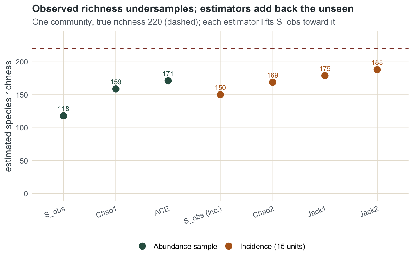
The bias shrinks with effort, but the floor does not lift
More individuals means fewer unseen species, so both the observed count and Chao1 climb toward the truth as the sample grows. The gap between them is the correction Chao1 supplies.
set.seed(6190)
Ns <- c(150, 300, 600, 1200); R <- 400
mc <- lapply(Ns, function(nn) {
  so <- ch <- numeric(R)
  for (r in 1:R) {
    cc <- as.vector(rmultinom(1, nn, rel)); o <- cc[cc > 0]
    so[r] <- length(o); ff <- tabulate(o)
    ff1 <- ff[1]; ff2 <- if (length(ff) >= 2) ff[2] else 0
    ch[r] <- length(o) + (nn - 1) / nn * ff1 * (ff1 - 1) / (2 * (ff2 + 1))
  }
  data.frame(N = nn, Sobs = mean(so), Chao1 = mean(ch))
})
mcdf <- do.call(rbind, mc); round(mcdf, 1)
N Sobs Chao1
1 150 67.2 122.2
2 300 96.3 142.8
3 600 126.0 164.6
4 1200 153.9 186.2mcl <- pivot_longer(mcdf, c(Sobs, Chao1), names_to = "quantity", values_to = "richness")
mcl$quantity <- factor(mcl$quantity, levels = c("Chao1","Sobs"),
labels = c("Chao1 (bias-corrected)", "observed S_obs"))
ggplot(mcl, aes(N, richness, colour = quantity)) +
geom_hline(yintercept = S_true, linetype = "dashed", colour = te["brick"], linewidth = 0.6) +
annotate("text", x = 160, y = S_true + 7, label = "true richness = 220",
colour = te["brick"], size = 3.3, hjust = 0) +
geom_line(linewidth = 0.9) + geom_point(size = 2.6) +
scale_x_log10(breaks = Ns) +
scale_colour_manual(values = c("Chao1 (bias-corrected)" = unname(te["forest"]),
"observed S_obs" = unname(te["sky"])), name = NULL) +
scale_y_continuous(limits = c(0, 235)) +
labs(title = "More sampling shrinks the gap, but Chao1 stays a lower bound",
subtitle = "Mean over 400 samples per sample size; Chao1 tracks below 220 throughout",
x = "individuals sampled (log scale)", y = "mean richness") +
theme_te()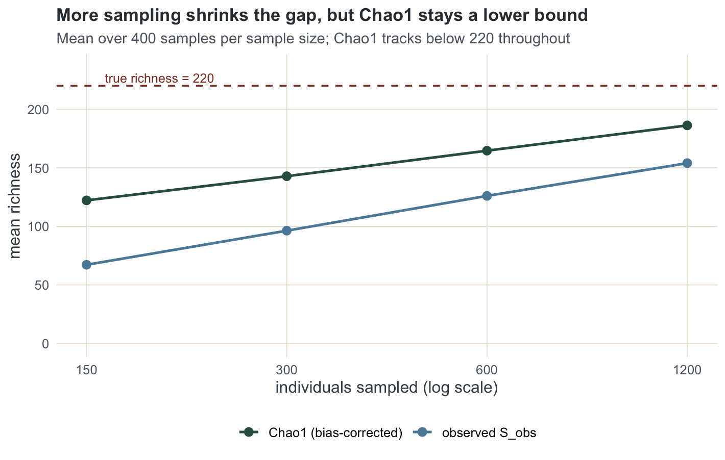
At 1200 individuals the observed count has reached 153.9 and Chao1 186.2, still short of 220. That is the honest limit. These estimators recover the species that the rare tail of your sample points to, and no more. When the community holds many species that are genuinely rare everywhere, the sample gives no signal about them, and a lower bound is the most you can defend. The next tutorial shows how to compare two such incomplete samples on equal terms.
References
Chao A 1984 Scandinavian Journal of Statistics 11(4):265-270 (no DOI, pre-DOI)
Chao A 1987 Biometrics 43(4):783-791 (10.2307/2531532)
Colwell R K, Coddington J A 1994 Philosophical Transactions of the Royal Society B 345(1311):101-118 (10.1098/rstb.1994.0091)
Gotelli N J, Colwell R K 2001 Ecology Letters 4(4):379-391 (10.1046/j.1461-0248.2001.00230.x)
Chiu C-H, Wang Y-T, Walther B A, Chao A 2014 Biometrics 70(3):671-682 (10.1111/biom.12200)
Magurran A E 2004 Measuring Biological Diversity (ISBN 978-0-632-05633-0)