library(ggplot2); library(dplyr); library(tidyr)
te <- c(forest = "#2f5d50", moss = "#7a9b76", rust = "#b5651d", gold = "#c9a227",
        slate = "#3d4b53", sand = "#d9cbb2", sky = "#5b8aa6", brick = "#8c3b2e")
theme_te <- function(base_size = 12) {
  theme_minimal(base_size = base_size) +
    theme(panel.grid.minor = element_blank(),
          panel.grid.major = element_line(colour = "#e7e1d5", linewidth = 0.3),
          axis.title = element_text(colour = "#3d4b53"),
          axis.text  = element_text(colour = "#5c6670"),
          plot.title = element_text(colour = "#2f3a40", face = "bold", size = base_size + 1),
          plot.subtitle = element_text(colour = "#5c6670", size = base_size - 1),
          legend.position = "bottom",
          legend.title = element_text(colour = "#3d4b53"),
          plot.background  = element_rect(fill = "#f5f4ee", colour = NA),
          panel.background = element_rect(fill = "#f5f4ee", colour = NA))
}Estimating diversity with Hill numbers
R
diversity
biodiversity
ecology tutorial
Plug-in Hill numbers are biased low under incomplete sampling, and the bias depends on the order q. Correct them in base R, and see why richness is the hardest.
Hill numbers give diversity a common currency: the effective number of equally common species, tuned by an order q that sets how much weight rare species carry. At q = 0 it is plain richness, at q = 1 it is the exponential of Shannon entropy, at q = 2 it is the inverse Simpson concentration. A companion post argues for reporting the whole profile rather than a single index. Here the question is different: given an incomplete sample, how well can you estimate each Hill number, and does the answer depend on q? It does, and the pattern is the point.
Hill numbers and their bias-corrected versions
The Hill number of order q is the reciprocal of the weighted power mean of order q - 1 of the species proportions, each proportion weighted by itself. Inverting is what puts the answer in units of species: a community of S equally common species returns S at every order. The naive, or plug-in, estimate just substitutes the observed proportions. Since those proportions come from an incomplete sample, the estimate is biased low, and there is a separate correction for each canonical order: Chao1 for richness, a Chao-Shen correction for Shannon, and an almost unbiased estimator for inverse Simpson.
hill <- function(p, q) { p <- p[p > 0]
  if (abs(q - 1) < 1e-9) exp(-sum(p * log(p))) else (sum(p^q))^(1 / (1 - q)) }
chao1 <- function(x) { n <- sum(x); f1 <- sum(x == 1); f2 <- sum(x == 2)
  length(x) + (n - 1) / n * f1 * (f1 - 1) / (2 * (f2 + 1)) }
covGT <- function(x) 1 - sum(x == 1) / sum(x)                    # Good-Turing coverage
shannon_CS <- function(x) { n <- sum(x); C <- covGT(x); pa <- C * (x / n)   # Chao-Shen
  -sum(pa * log(pa) / (1 - (1 - pa)^n)) }
simpson_hat <- function(x) { n <- sum(x); 1 / sum(x * (x - 1) / (n * (n - 1))) }  # unbiased
A community and a sample
The true community holds 160 species; we draw 300 individuals.
set.seed(4192)
S_true <- 160
rel <- exp(rnorm(S_true, 0, 1.5)); rel <- rel / sum(rel)
n <- 300
x <- as.vector(rmultinom(1, n, rel)); x <- x[x > 0]
Sobs <- length(x); phat <- x / n
c(S_true = S_true, S_obs = Sobs, coverage = round(covGT(x), 4))
S_true S_obs coverage
160.00 77.00 0.87 The sample sees 77 of 160 species, at a coverage of 0.87. Now compare the truth, the plug-in estimate and the bias-corrected estimate at each order.
truD <- c(hill(rel, 0),  hill(rel, 1),  hill(rel, 2))
empD <- c(hill(phat, 0), hill(phat, 1), hill(phat, 2))
estD <- c(chao1(x),      exp(shannon_CS(x)), simpson_hat(x))
data.frame(q = c(0, 1, 2), true = round(truD, 1),
           empirical = round(empD, 1), estimated = round(estD, 1),
           rel_bias_empirical = round((empD - truD) / truD, 3))
q true empirical estimated rel_bias_empirical
1 0 160.0 77.0 133.8 -0.519
2 1 42.9 36.6 46.7 -0.146
3 2 22.2 20.9 22.4 -0.060At q = 0 the plug-in estimate is 77 against a truth of 160, a relative bias of -52 per cent, because richness counts every species equally and the unseen ones are all missing. Chao1 lifts it to 133.8, much better but still a lower bound. At q = 1 the plug-in bias is only -15 per cent and the Chao-Shen correction lands at 46.7, close to the truth of 42.9. At q = 2 the plug-in estimate is already within 6 per cent, and the unbiased estimator returns 22.4 against 22.2.
The whole profile
Plotting the full profile makes the gradient in bias obvious: the plug-in curve hugs the truth at high q and peels away as q falls to zero.
qgrid <- seq(0, 3, by = 0.1)
prof <- data.frame(q = rep(qgrid, 2),
  D = c(sapply(qgrid, function(q) hill(rel, q)),
        sapply(qgrid, function(q) hill(phat, q))),
  series = rep(c("true", "empirical (plug-in)"), each = length(qgrid)))
estpts <- data.frame(q = c(0, 1, 2), D = estD)
ggplot(prof, aes(q, D, colour = series, linetype = series)) +
  geom_line(linewidth = 0.9) +
  geom_point(data = estpts, aes(q, D), inherit.aes = FALSE,
             colour = te["rust"], size = 3.4, shape = 17) +
  annotate("text", x = 0.08, y = truD[1] + 8, label = "richness (q = 0): biggest gap",
           hjust = 0, size = 3.1, colour = te["slate"]) +
  scale_colour_manual(values = c("true" = unname(te["forest"]),
                                 "empirical (plug-in)" = unname(te["sky"]),
                                 "estimated (bias-corrected)" = unname(te["rust"])), name = NULL) +
  scale_linetype_manual(values = c("true" = "solid", "empirical (plug-in)" = "22",
                                   "estimated (bias-corrected)" = "solid"), name = NULL) +
  labs(title = "The plug-in diversity profile is biased low, worst at q = 0",
       subtitle = "One community, true S = 160, n = 300; triangles are bias-corrected estimates at q = 0, 1, 2",
       x = "diversity order q", y = "Hill number (effective species)") +
  theme_te()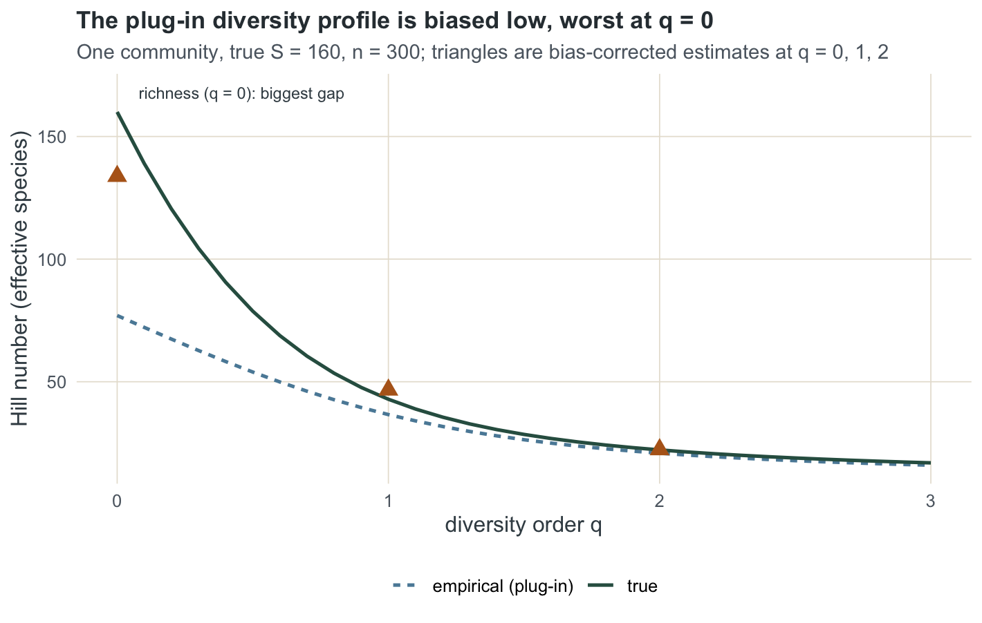
The bias is systematic, and estimability follows q
A single sample could be lucky. Repeating the draw shows the bias is a property of the estimator, not the draw, and that it collapses as q rises.
set.seed(5192); R <- 500
mat <- replicate(R, { xx <- as.vector(rmultinom(1, n, rel)); xx <- xx[xx > 0]; pp <- xx / sum(xx)
  c(hill(pp, 0), hill(pp, 1), hill(pp, 2),
    chao1(xx), exp(shannon_CS(xx)), simpson_hat(xx)) })
mm <- rowMeans(mat)
mcbias <- data.frame(q = c(0, 1, 2),
  rb_emp = (mm[1:3] - truD) / truD,
  rb_est = (mm[4:6] - truD) / truD)
round(mcbias, 3)
q rb_emp rb_est
1 0 -0.572 -0.346
2 1 -0.198 -0.016
3 2 -0.061 0.006mbl <- data.frame(q = factor(rep(c(0, 1, 2), 2)),
rbias = c(mcbias$rb_emp, mcbias$rb_est),
method = rep(c("empirical (plug-in)", "estimated (bias-corrected)"), each = 3))
ggplot(mbl, aes(q, rbias, fill = method)) +
geom_hline(yintercept = 0, colour = te["slate"], linewidth = 0.4) +
geom_col(position = position_dodge(width = 0.7), width = 0.6) +
geom_text(aes(label = sprintf("%+.0f%%", 100 * rbias)),
position = position_dodge(width = 0.7),
vjust = ifelse(mbl$rbias < 0, 1.3, -0.5), size = 2.9, colour = te["slate"]) +
scale_fill_manual(values = c("empirical (plug-in)" = unname(te["sky"]),
"estimated (bias-corrected)" = unname(te["rust"])), name = NULL) +
scale_y_continuous(labels = scales::percent, limits = c(-0.65, 0.12)) +
labs(title = "Estimability of diversity depends on the order q",
subtitle = "Mean relative bias over 500 samples; the plug-in gap collapses as q rises, q = 0 stays hardest",
x = "diversity order q", y = "relative bias") +
theme_te()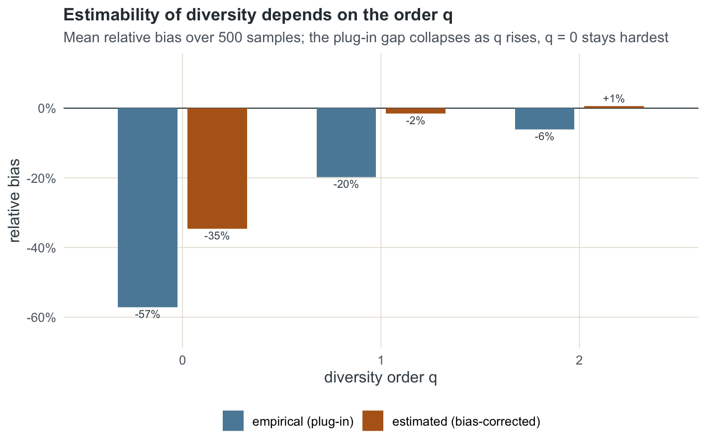
The plug-in bias runs from -57 per cent at q = 0 to about -6 per cent at q = 2. Correction nearly erases it for q = 1 and q = 2, at -2 and +1 per cent, but richness stays stubborn: even the corrected estimate at q = 0 is 35 per cent low, because it is still a lower bound leaning on the unseen tail.
Why q sets the difficulty
Diversity is not one quantity to estimate but a family, and the family splits by how much it depends on species you may never see. High-order diversities weight the common species, which any decent sample captures, so they are close to unbiased and easy to estimate. Richness weights every species equally, including the ones that leave no trace, so it is the most sensitive to sampling and the hardest to pin down. When someone quotes a single diversity number from a sample, the order q behind it tells you how much to trust it. The final post in this cluster turns these estimates over and asks what checks reveal about their reliability.
References
Hill M O 1973 Ecology 54(2):427-432 (10.2307/1934352)
Jost L 2006 Oikos 113(2):363-375 (10.1111/j.2006.0030-1299.14714.x)
Jost L 2007 Ecology 88(10):2427-2439 (10.1890/06-1736.1)
Chao A, Shen T-J 2003 Environmental and Ecological Statistics 10:429-443 (10.1023/A:1026096204727)
Chao A, Gotelli N J, Hsieh T C, Sander E L, Ma K H, Colwell R K, Ellison A M 2014 Ecological Monographs 84(1):45-67 (10.1890/13-0133.1)
Roswell M, Dushoff J, Winfree R 2021 Oikos 130(3):321-338 (10.1111/oik.07202)