library(vegan)
library(ggplot2)

paper <- "#f5f4ee"; ink <- "#16241d"; forest <- "#275139"
gold  <- "#cda23f"; abandoned <- "#b5534e"; faint <- "#5d6b61"; line <- "#dad9ca"

theme_te <- theme_minimal(base_size = 12) +
  theme(panel.grid.minor = element_blank(),
        panel.grid.major = element_line(colour = line, linewidth = 0.3),
        plot.background = element_rect(fill = paper, colour = NA),
        panel.background = element_rect(fill = paper, colour = NA),
        axis.title = element_text(colour = ink),
        axis.text = element_text(colour = faint),
plot.title = element_text(colour = ink, face = "bold"))When not to use the Shannon diversity index
diversity
ecology tutorial
vegan
R
The Shannon index blends richness and evenness into one number, which can mislead. When Hill numbers, evenness, or richness tell a clearer ecological story.
The Shannon index is the reflex choice for summarising diversity, and that is part of the problem. It compresses two distinct properties of a community, how many species are present and how evenly the individuals are spread among them, into a single number. When those two properties move together the summary is fine. When they move in opposite directions, a single Shannon value can hide the very difference you are trying to detect, and can even rank communities backwards. This post shows that failure with a worked example, then points to the tools that keep richness and evenness visible.
Two communities, one misleading number
Consider two sampled communities. Community A is species-rich but dominated by one abundant species. Community B has fewer species but spreads its individuals almost evenly.
A <- c(50, 25, 12, 6, 3, 2, 1, 1)   # 8 species, uneven
B <- c(22, 20, 19, 18, 16)          # 5 species, even

H <- function(x) { p <- x / sum(x); -sum(p * log(p)) }

c(shannon_A = H(A), shannon_B = H(B),
  richness_A = sum(A > 0), richness_B = sum(B > 0),
  evenness_A = H(A) / log(sum(A > 0)),
  evenness_B = H(B) / log(sum(B > 0)))
shannon_A shannon_B richness_A richness_B evenness_A evenness_B
1.3919240 1.6038766 8.0000000 5.0000000 0.6693740 0.9965445 Community A holds eight species, Community B only five, so A is plainly richer. Yet its Shannon index, 1.39, is lower than B’s 1.6. By Shannon alone you would call B the more diverse community and never learn that A has more species. The reason sits in the evenness column: A’s Pielou evenness is 0.67 against B’s 1. Shannon weighs evenness heavily, so B’s near-perfect balance outweighs A’s extra species. Whether that is the right conclusion depends entirely on the ecological question, and the single number does not let you ask it.
Hill numbers keep both properties visible
The cleaner approach reports diversity as a function of one parameter, the order q, which sets how much rare species count. Hill numbers express each value as an effective number of species, the number of equally-common species that would give the same diversity. At q = 0 rare species count fully and the Hill number is simply richness. At q = 1 species count in proportion to their abundance, which is the exponential of the Shannon index. At q = 2 common species dominate, giving the inverse Simpson concentration. Plotting the whole profile shows the trade-off directly.
qfull <- seq(0, 3, by = 0.05)
prof <- rbind(
  data.frame(q = qfull, D = as.numeric(renyi(A, scales = qfull, hill = TRUE)),
             community = "A: rich, uneven"),
  data.frame(q = qfull, D = as.numeric(renyi(B, scales = qfull, hill = TRUE)),
             community = "B: poor, even")
)

ggplot(prof, aes(q, D, colour = community)) +
  geom_line(linewidth = 1) +
  geom_vline(xintercept = 0.6, colour = faint, linetype = "dashed", linewidth = 0.4) +
  scale_colour_manual(values = c("A: rich, uneven" = abandoned,
                                 "B: poor, even" = forest)) +
  labs(x = "order q (weight on common species)",
       y = "effective number of species",
       colour = NULL, title = "Which community is more diverse? It depends on q") +
  theme_te + theme(legend.position = "top")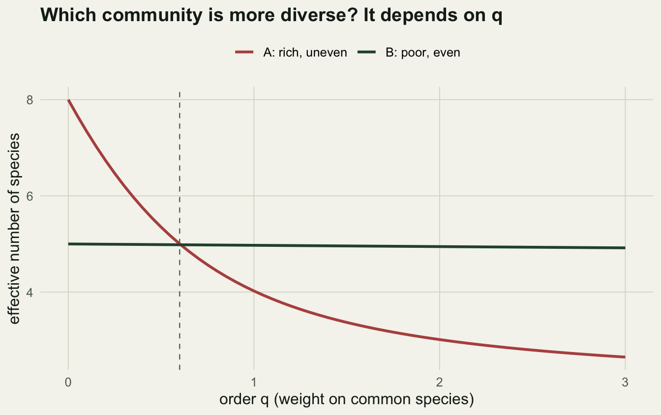
The crossing is the whole point. At q = 0 community A leads, because it has more species. By q = 2 community B leads, because its individuals are evenly distributed. A single index picks one point on the horizontal axis and pretends the rest does not exist. Reporting the profile, or at least the trio of richness, exponential Shannon, and inverse Simpson, makes the trade-off explicit and reproducible.
Shannon also shifts with sample size
A second, quieter trap: the Shannon index is biased downward in small samples, because rare species go undetected and the estimate of evenness is distorted. Subsample one community at increasing effort and the estimate drifts upward toward its true value.
set.seed(88)
pool <- rep(seq_along(A), A * 40)        # large community with A's proportions
subsizes <- c(20, 50, 100, 300, 800)
res <- data.frame(
  n = subsizes,
  H = sapply(subsizes, function(n) {
    mean(replicate(200, { s <- sample(pool, n); p <- table(s) / n; -sum(p * log(p)) }))
  })
)

ggplot(res, aes(n, H)) +
  geom_hline(yintercept = H(A), colour = faint, linetype = "dashed") +
  geom_line(colour = gold, linewidth = 1) + geom_point(colour = gold, size = 2) +
  scale_x_log10(breaks = subsizes) +
  labs(x = "subsample size (log scale)", y = "estimated Shannon index",
       title = "Shannon drifts upward with sampling effort") +
  theme_te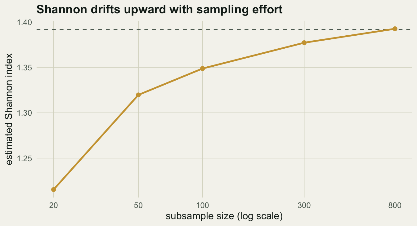
The estimate starts near 1.22 at twenty individuals and only reaches the true 1.39 after several hundred. If two sites were sampled with different effort, a difference in Shannon could be nothing more than a difference in how hard you looked.
What to do instead
None of this means abandoning Shannon, which is a reasonable q = 1 summary when communities are sampled comparably and you want one evenness-sensitive number. It means not leaning on it alone. Report richness and an evenness measure separately, so the two properties stay legible. Better still, report Hill numbers at q = 0, 1, and 2, or the full diversity profile, which expresses everything in the same interpretable unit of effective species and reveals crossings a single index would bury. And when comparing across samples, standardise the effort first, by rarefaction or coverage, so the comparison is of diversity rather than of sampling. The extra columns cost almost nothing and stop a single number from quietly making the decision for you.
References
Hill MO 1973 Ecology 54(2):427-432 (10.2307/1934352)
Jost L 2006 Oikos 113(2):363-375 (10.1111/j.2006.0030-1299.14714.x)