Species richness, Shannon and Simpson from a community matrix, with code you can reuse.
Author
Tidy Ecology
Published
2026-06-18
Alpha diversity, meaning how diverse a single site or sample is, is usually the first number an ecologist wants out of a species-abundance table. This post covers the three you’ll reach for most often: species richness, the Shannon index, and the Simpson index, all from the vegan package.
We’ll go from a raw community matrix to a tidy results table and a finished plot.
A community matrix
vegan expects a community matrix: one row per site (or sample), one column per species, cells holding abundances (counts or cover). Here’s a small worked example, with counts of five plant species across four meadow plots:
Each row is a plot; each column a species. Plot_C is dominated by Festuca, while Plot_D spreads its individuals evenly across all five species.
The three indices
vegan gives you each of these in a single call:
richness <-specnumber(community) # number of species presentshannon <-diversity(community, index ="shannon")simpson <-diversity(community, index ="simpson")richness
specnumber() simply counts the non-zero species. It’s the most basic measure, and blind to abundance.
Shannon (H′) rises with both richness and evenness; for real communities it usually falls between about 1.5 and 3.5.
Simpson is returned here as 1 − D: the probability that two individuals drawn at random belong to different species. It runs from 0 to 1 and is less sensitive to rare species than Shannon.
A tidy results table
Let’s pull everything into one data frame, rounded for reading:
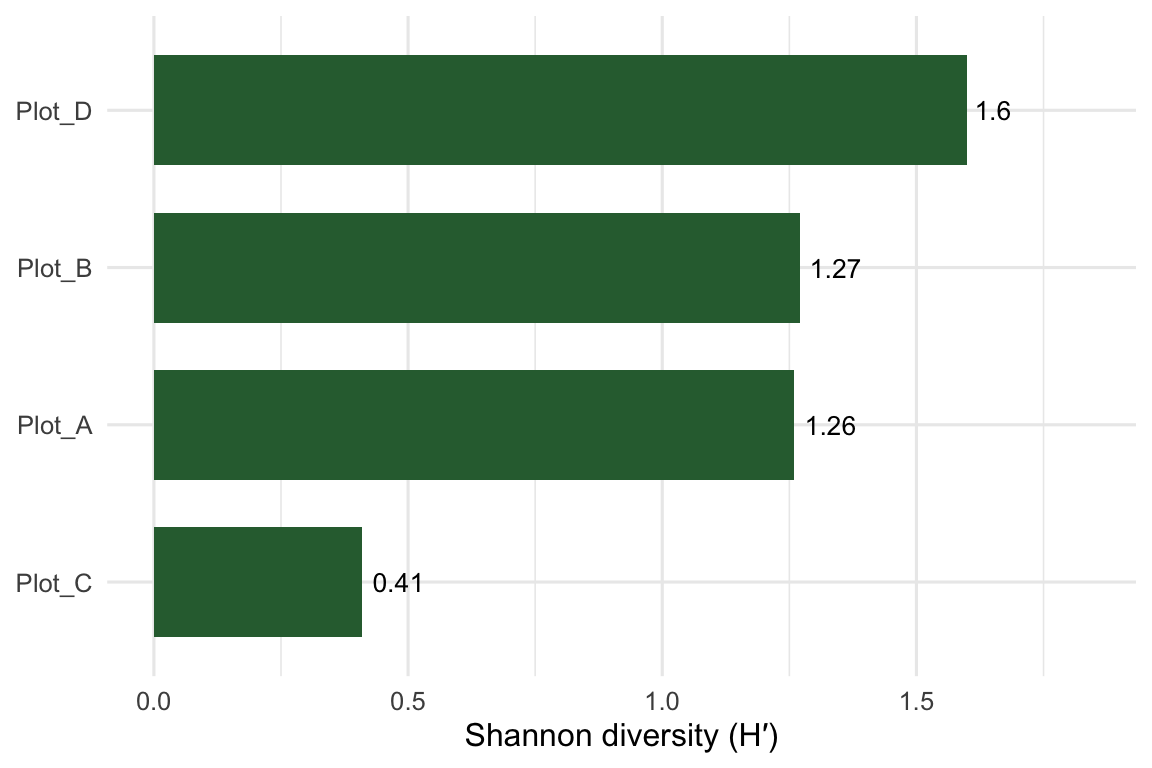
Plot_D comes out most diverse. It carries all five species at similar abundances, so its evenness is high. Plot_A and Plot_B land in the middle and almost tie (1.26 vs 1.27), despite very different species makeups. Plot_C, dominated by a single grass, scores lowest even though three species are present. That gap between richness and Shannon is the evenness effect at work.
A plot
Finally, the bit you’ll actually paste into a report: Shannon diversity per plot.
Figure 1: Shannon diversity (H′) across the four meadow plots.
Where to go next
This is the foundation. Realistic next steps:
swap the toy matrix for your own data, read in with read.csv() into the same site-by-species shape;
add Pielou’s evenness (shannon / log(richness)) to separate richness from evenness explicitly;
once you have many sites, move from alpha to beta diversity and ordination (vegdist(), metaMDS()).
Ordination is the next post. If you hit a snag adapting this to your own data, let me know.
Source Code
---title: "Computing diversity indices in R with vegan"description: "Species richness, Shannon and Simpson from a community matrix, with code you can reuse."date: "2026-06-18"categories: [R, biodiversity, tutorial]---Alpha diversity, meaning how diverse a single site or sample is, is usually the first number an ecologist wants out of a species-abundance table. This post covers the three you'll reach for most often: **species richness**, the **Shannon index**, and the **Simpson index**, all from the `vegan` package.We'll go from a raw community matrix to a tidy results table and a finished plot.## A community matrix`vegan` expects a **community matrix**: one row per site (or sample), one column per species, cells holding abundances (counts or cover). Here's a small worked example, with counts of five plant species across four meadow plots:```{r}#| label: community-matrix#| message: falselibrary(vegan)library(dplyr)library(ggplot2)community <-data.frame(row.names =c("Plot_A", "Plot_B", "Plot_C", "Plot_D"),Festuca =c(10, 0, 25, 4),Trifolium =c( 8, 12, 2, 5),Plantago =c( 5, 3, 1, 6),Achillea =c( 2, 9, 0, 5),Lotus =c( 0, 15, 0, 4))community```Each row is a plot; each column a species. `Plot_C` is dominated by *Festuca*, while `Plot_D` spreads its individuals evenly across all five species.## The three indices`vegan` gives you each of these in a single call:```{r}#| label: compute-indicesrichness <-specnumber(community) # number of species presentshannon <-diversity(community, index ="shannon")simpson <-diversity(community, index ="simpson")richnessshannonsimpson```A few things worth knowing:- **`specnumber()`** simply counts the non-zero species. It's the most basic measure, and blind to abundance.- **Shannon (H′)** rises with both richness *and* evenness; for real communities it usually falls between about 1.5 and 3.5.- **Simpson** is returned here as 1 − D: the probability that two individuals drawn at random belong to *different* species. It runs from 0 to 1 and is less sensitive to rare species than Shannon.## A tidy results tableLet's pull everything into one data frame, rounded for reading:```{r}#| label: results-tablediversity_summary <-tibble(plot =rownames(community),richness = richness,shannon =round(shannon, 2),simpson =round(simpson, 2)) |>arrange(desc(shannon))diversity_summary````Plot_D` comes out most diverse. It carries all five species at similar abundances, so its evenness is high. `Plot_A` and `Plot_B` land in the middle and almost tie (1.26 vs 1.27), despite very different species makeups. `Plot_C`, dominated by a single grass, scores lowest even though three species are present. That gap between *richness* and *Shannon* is the evenness effect at work.## A plotFinally, the bit you'll actually paste into a report: Shannon diversity per plot.```{r}#| label: fig-shannon#| fig-cap: "Shannon diversity (H′) across the four meadow plots."#| fig-width: 6#| fig-height: 4ggplot(diversity_summary, aes(x =reorder(plot, shannon), y = shannon)) +geom_col(fill ="#2f6b3e", width =0.7) +geom_text(aes(label = shannon), hjust =-0.2, size =3.5) +coord_flip() +labs(x =NULL, y ="Shannon diversity (H′)") +ylim(0, max(diversity_summary$shannon) *1.15) +theme_minimal(base_size =12)```## Where to go nextThis is the foundation. Realistic next steps:- swap the toy matrix for your own data, read in with `read.csv()` into the same site-by-species shape;- add **Pielou's evenness** (`shannon / log(richness)`) to separate richness from evenness explicitly;- once you have many sites, move from alpha to **beta diversity** and ordination (`vegdist()`, `metaMDS()`).Ordination is the next post. If you hit a snag adapting this to your own data, [let me know](../../contact.qmd).