From a field sheet to your first analysis

A worked R pipeline for ecologists: read a messy field sheet, clean species names, reshape and join, then compute diversity, letting cleaning decide the result.

The earlier tutorials in this series each fixed one problem: a blank cell is not a zero, a species table can be wide or long, name variants inflate richness, and an inner join drops absent sites. This post runs the whole pipeline end to end on one messy field sheet, so you can see how the pieces connect and, more importantly, how the cleaning steps decide the answer. We finish with a first diversity analysis and hand off to the diversity tutorial for what the numbers mean.

The measurable point of a worked example is that the decisions compound. Skipping the name cleaning and using the wrong join does not just shift a number: it changes which site you would call the most diverse.

The raw sheet

Field sheets are typed by people, so they are messy. Here is one as it might come out of a spreadsheet: long format, one row per record, with the species names entered inconsistently (mixed case and a stray double space) because different people wrote them on different days:

library(dplyr)
library(tidyr)
raw_csv <- "site,species,count
S1,Carex flava,20
S1,Carex flacca,8
S1,Juncus effusus,5
S1,Poa pratensis,3
S2,Carex flava,15
S2,Juncus effusus,20
S2,Festuca rubra,10
S3,Carex flava,10
S3,carex flava,10
S3,Carex  flava,10
S3,Poa pratensis,10"
raw <- read.csv(text = raw_csv, stringsAsFactors = FALSE)
raw

   site        species count
1    S1    Carex flava    20
2    S1   Carex flacca     8
3    S1 Juncus effusus     5
4    S1  Poa pratensis     3
5    S2    Carex flava    15
6    S2 Juncus effusus    20
7    S2  Festuca rubra    10
8    S3    Carex flava    10
9    S3    carex flava    10
10   S3   Carex  flava    10
11   S3  Poa pratensis    10

We also have a survey frame: the list of every site that was visited. Four sites were surveyed, and site S4 turned up no plants at all, so it never appears in the observations:

sites <- data.frame(
  site    = paste0("S", 1:4),
  habitat = c("fen", "fen", "meadow", "meadow"),
  stringsAsFactors = FALSE
)
sites

  site habitat
1   S1     fen
2   S2     fen
3   S3  meadow
4   S4  meadow

Look at S3. The three rows Carex flava, carex flava and Carex flava are the same species written three ways. Uncorrected, R treats them as three species. That is the trap the pipeline has to close.

A helper for the diversity index

We will compute the Shannon index, which needs relative abundances. This one-line helper takes a vector of counts and returns Shannon diversity (it drops zeros, since 0 * log(0) is defined as zero):

shannon <- function(x) {
  p <- x[x > 0]
  p <- p / sum(p)
  -sum(p * log(p))
}

The naive pipeline

First, the pipeline a hurried analyst writes: sum counts per site and species, pivot to a wide site-by-species matrix, and join the survey frame with an inner join. No name cleaning:

naive_wide <- raw |>
  group_by(site, species) |>
  summarise(count = sum(count), .groups = "drop") |>
  pivot_wider(names_from = species, values_from = count, values_fill = 0)

naive <- naive_wide |>
  rowwise() |>
  mutate(richness = sum(c_across(-site) > 0),
         shannon  = shannon(c_across(-c(site, richness)))) |>
  ungroup() |>
  select(site, richness, shannon)

# inner join with the survey frame: S4 has no observations, so it is dropped
naive_out <- inner_join(sites, naive, by = "site")
naive_out |> mutate(shannon = round(shannon, 3))

  site habitat richness shannon
1   S1     fen        4   1.142
2   S2     fen        3   1.061
3   S3  meadow        4   1.386

By this account the most diverse site is S3, with a Shannon value of 1.386 and a richness of 4. That is entirely an artefact: S3’s three spellings of Carex flava became three equally abundant species, which is the most even four-species community possible.

The clean pipeline

Now the careful version. We normalise the names first (trim whitespace, collapse internal spaces, lower-case), map them through a small lookup so every variant resolves to one accepted name, and check that nothing fell through. Then the same reshape, but with a left join so the surveyed-but-empty S4 is kept and its missing counts become zeros:

normalise <- function(x) tolower(gsub("\\s+", " ", trimws(x)))
lookup <- c("carex flava"    = "Carex flava",
            "carex flacca"   = "Carex flacca",
            "juncus effusus" = "Juncus effusus",
            "poa pratensis"  = "Poa pratensis",
            "festuca rubra"  = "Festuca rubra")

raw_clean <- raw |> mutate(species = lookup[normalise(species)])
stopifnot(!anyNA(raw_clean$species))   # every raw string matched the lookup

clean_wide <- raw_clean |>
  group_by(site, species) |>
  summarise(count = sum(count), .groups = "drop") |>
  pivot_wider(names_from = species, values_from = count, values_fill = 0)

clean <- clean_wide |>
  rowwise() |>
  mutate(richness = sum(c_across(-site) > 0),
         shannon  = shannon(c_across(-c(site, richness)))) |>
  ungroup() |>
  select(site, richness, shannon)

# left join keeps S4 (surveyed, nothing found): richness 0, Shannon 0
clean_out <- left_join(sites, clean, by = "site") |>
  mutate(richness = replace_na(richness, 0L),
         shannon  = replace_na(shannon, 0))
clean_out |> mutate(shannon = round(shannon, 3))

  site habitat richness shannon
1   S1     fen        4   1.142
2   S2     fen        3   1.061
3   S3  meadow        2   0.562
4   S4  meadow        0   0.000

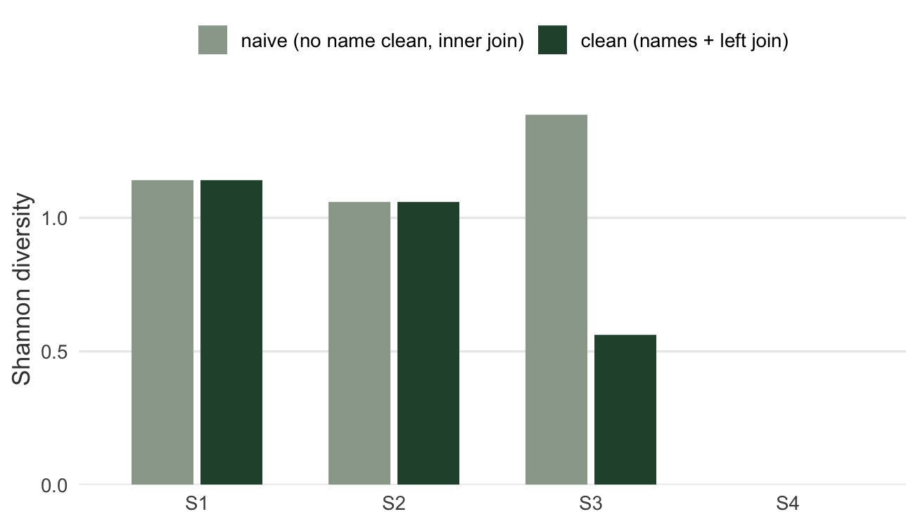
Two things move. S3’s richness falls from 4 to 2 and its Shannon value from 1.386 to 0.562, once its three fake species collapse into one real Carex flava. And S4 reappears as a surveyed site with zero plants. The most diverse site is now S1, not S3.

The decisions compounded

Put the two pipelines side by side and the effect is not subtle:

Figure 1: Shannon diversity by site under the naive pipeline (no name cleaning, inner join) and the clean pipeline. Uncorrected name variants make S3 look like the most diverse site; cleaning them collapses S3 and puts S1 on top, and the left join restores the surveyed-but-empty S4.

The mean richness across sites tells the same story from the summary side: the naive pipeline reports 3.67 species per site over 3 sites, while the clean pipeline reports 2.25 over 4 sites. Both the inflation (name variants adding species) and the deflation (the dropped empty site) come from cleaning decisions, not from the plants.

Where to go next

You now have a clean site-by-species matrix and a first diversity number per site. What Shannon actually measures, how it trades off richness against evenness, and when a different index is a better choice, is the subject of the alpha-diversity tutorial. Everything downstream, ordination, models, maps, starts from the same clean table you just built.

Related tutorials

• Reading field data into R
• Cleaning species names before you count
• Joining ecological tables without losing zeros
• Alpha diversity indices in R

References

Wickham H 2014. Journal of Statistical Software 59(10):1 (10.18637/jss.v059.i10).

Gotelli NJ, Colwell RK 2001. Ecology Letters 4(4):379 (10.1046/j.1461-0248.2001.00230.x).