---
title: "Cleaning species names before you count"
description: "One species written six ways becomes six species in your richness count. Clean names with trimws, tolower and a lookup table before fuzzy matching traps you."
date: "2026-06-18 12:00"
date-modified: "2026-10-14"
categories: [R, data import, community ecology, biodiversity, ecology tutorial]
image: thumbnail.png
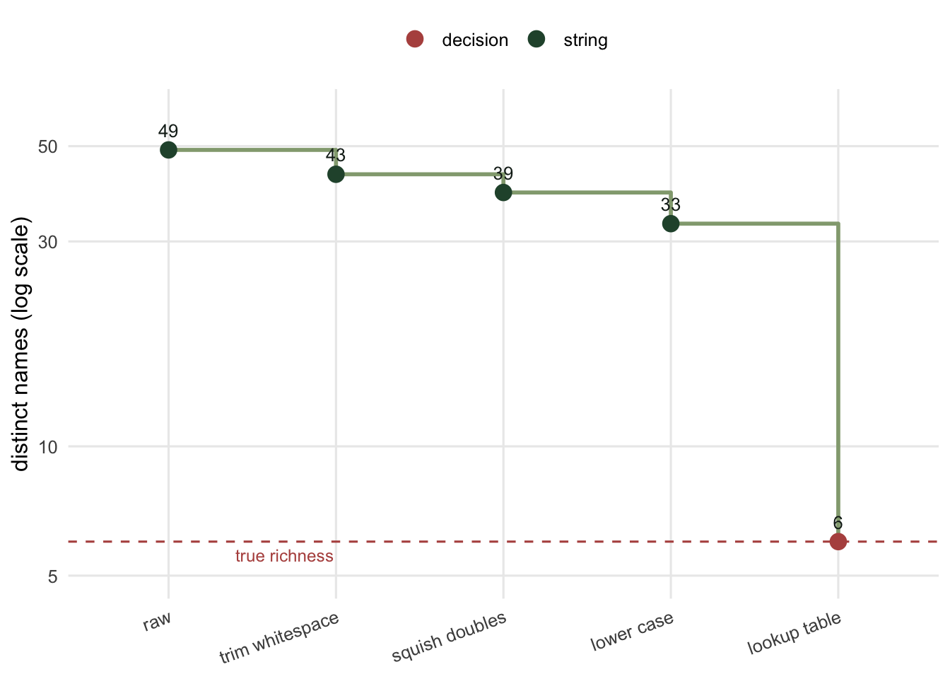
image-alt: "A step chart falling from forty-nine distinct recorded names down to six, with most of the drop coming from a lookup table rather than from string tidying."
---
*Corrected 14 October 2026: the post said that the order of the three string operations shapes the funnel because whichever runs first takes credit for variants that two of them could catch; no variant here can be caught by two of them, so each operation removes the same number of names in any order, and the text now says that the order only rearranges the steps.*
*Corrected 7 October 2026: the post said the three string operations remove most of the variant names, when they clear just over a third of the excess, and it left appended authorities out of the variants that survive them; the caption of the effort figure also still described true richness as nearly flat and the whole gradient as a typo gradient, and it now matches the correction below.*
*Corrected 30 September 2026: the post said the typos manufactured an effort gradient in richness that is not in the data; true richness also rises with effort, so the text now says the typos make that gradient far steeper, and that the extra strength, not the whole relationship, is an artefact.*
`length(unique(species))` is the first line of almost every diversity analysis, and it trusts the spelling completely. Write *Festuca rubra* one day and *festuca rubra* the next, add a stray space, let someone abbreviate it to *F. rubra*, and R counts four species where the field held one. Nobody decided this; it is the sum of small keystrokes across a season, and it inflates richness in exactly the plots where you worked hardest.
This post takes one messy notebook, cleans it in the order that actually works, and stops at the point where string tidying can do no more. The last step is a lookup table, and the tempting shortcut past it, fuzzy matching, is where the real damage happens.
## One notebook, many spellings
The notebook below is synthetic: twelve plots, six real species, and a realistic rate of transcription slips. The generator is in the source; what matters is the column it produced, which is what a shared field sheet looks like after a season of hands.
```{r make-nb}
#| code-fold: true
#| code-summary: "Code behind this output; later chunks use it, so run it first"
set.seed(317)

pool <- c("Festuca rubra", "Trifolium pratense", "Plantago lanceolata",
          "Achillea millefolium", "Carex flacca", "Carex flava")
authority <- setNames(c("L.", "L.", "L.", "L.", "Schreb.", "L."), pool)
prob <- c(0.34, 0.20, 0.16, 0.14, 0.09, 0.07)

swap_letters <- function(x) {
  ch <- strsplit(x, "")[[1]]
  ok <- which(ch != " " & c(ch[-1], "") != " ")
  ok <- ok[ok < length(ch)]
  i <- sample(ok, 1)
  ch[c(i, i + 1)] <- ch[c(i + 1, i)]
  paste(ch, collapse = "")
}
mistype <- function(x) {
  switch(sample(6, 1),
         tolower(x),
         paste0(x, " "),
         sub(" ", "  ", x),
         swap_letters(x),
         sub("^(.)[a-z]+ ", "\\1. ", x),
         paste(x, authority[[x]]))
}

effort <- c(5, 7, 9, 12, 15, 18, 22, 27, 33, 40, 50, 60)
plots <- paste0("P", sprintf("%02d", seq_along(effort)))

nb <- do.call(rbind, lapply(seq_along(effort), function(i) {
  sp <- sample(pool, effort[i], replace = TRUE, prob = prob)
  typed <- vapply(sp, function(s) if (runif(1) < 0.30) mistype(s) else s, character(1))
  data.frame(plot = plots[i], recorded = unname(typed), true_name = sp)
}))
```
```{r peek}
head(nb[, c("plot", "recorded")], 8)
nrow(nb)
```
Now the line that starts every analysis, run on the column as typed:
```{r headline}
length(unique(nb$recorded))
```
`r length(unique(nb$recorded))` species, from a field that held six. Here they are, and every one is a variant of the same six binomials:
```{r all-variants}
sort(unique(nb$recorded))
```
Trailing spaces, double spaces, lower case, transposed letters, abbreviations, appended authorities. Each is a different string to R, and `unique()` has no way to know they are the same plant.
## Clean the whitespace and the case
Three string operations remove the whitespace and case variants, though most of the excess names survive them. Run them one at a time so you can watch the count fall.
```{r chain}
x <- nb$recorded
step <- c(raw = length(unique(x)))

x <- trimws(x)
step["trim whitespace"] <- length(unique(x))

x <- gsub("\\s+", " ", x)
step["squish doubles"] <- length(unique(x))

x <- tolower(x)
step["lower case"] <- length(unique(x))

step
```
`trimws` strips the leading and trailing spaces, `gsub("\\s+", " ", x)` collapses any run of internal whitespace to one space, and `tolower` removes the capitalisation differences. The three commute: none of them can reintroduce what another removed, so any order lands on the same set of cleaned strings. What the order does change is the shape of the funnel below, though not the size of each step: each slip here is a single change that at most one of the three operations can undo, so each operation removes the same number of names wherever it runs, and the order only rearranges the steps.
```{r fig-funnel}
#| fig-cap: "The distinct name count after each cleaning operation. Whitespace and case tidying remove a lot, but the count settles well above the six species that were actually present. The last drop, from the plateau down to six, is not a string operation at all; it is a decision about which spellings mean which species."
#| fig-alt: "A step chart on a log scale. The count falls from forty-nine at raw, to forty-three after trimming, thirty-nine after squishing, thirty-three after lower casing, then a large final step down to six labelled lookup table. A dashed line marks the true richness of six."
library(ggplot2)
te_canvas <- theme(plot.background  = element_rect(fill = "#f5f4ee", colour = NA),
                   panel.background = element_rect(fill = "#f5f4ee", colour = NA))

steps <- data.frame(
  stage = factor(c(names(step), "lookup table"), levels = c(names(step), "lookup table")),
  n = c(step, 6),
  kind = c("string", "string", "string", "string", "decision")
)

ggplot(steps, aes(stage, n, group = 1)) +
  geom_hline(yintercept = 6, linetype = "dashed", colour = "#b5534e") +
  geom_step(colour = "#93a87f", linewidth = 1) +
  geom_point(aes(colour = kind), size = 3.6) +
  geom_text(aes(label = n, hjust = ifelse(stage == "lookup table", 1.3, -0.4)),
            vjust = -0.5, size = 3.4, colour = "#16241d") +
  annotate("text", x = 1.4, y = 6, label = "true richness", vjust = 1.6,
           colour = "#b5534e", size = 3.2, hjust = 0) +
  scale_colour_manual(values = c(string = "#275139", decision = "#b5534e")) +
  scale_y_log10(limits = c(5, 60)) +
  labs(x = NULL, y = "distinct names (log scale)", colour = NULL) +
  theme_minimal(base_size = 12) + te_canvas +
  theme(legend.position = "top", panel.grid.minor = element_blank(),
        axis.text.x = element_text(angle = 20, hjust = 1))
```
The chain gets from `r step["raw"]` to `r step["lower case"]`. That clears `r sprintf("%d", step["raw"] - step["lower case"])` of the `r sprintf("%d", step["raw"] - 6)` names in excess of the true six, about `r sprintf("%.0f", 100 * (step["raw"] - step["lower case"]) / (step["raw"] - 6))` per cent of the gap, and it is where a lot of analyses stop. It is also still `r step["lower case"] - 6` species too many, and no amount of further string tidying closes the gap, because the remaining variants are not typos of layout. They are abbreviations, misspellings and appended authorities, and while a further string rule could strip the authorities, *f. rubra* is not mechanically closer to *festuca rubra* than it is to anything else.
## The lookup table is the honest tool
The remaining `r step["lower case"]` strings have to be mapped to accepted names by a decision, one row per variant, written down where it can be checked.
```{r lookup-build}
clean <- tolower(gsub("\\s+", " ", trimws(nb$recorded)))

lookup <- data.frame(recorded = sort(unique(clean)))
head(lookup, 6)
```
For a real dataset you write the accepted name beside each variant by hand, or against a taxonomic authority. Since this notebook is synthetic, we already know the intended species for every record, so we can build the map from that and see the result:
```{r lookup-apply}
key <- tapply(tolower(nb$true_name), clean, function(v) v[1])
accepted <- unname(key[clean])
length(unique(accepted))
```
Six. The lookup is the step that reached the truth, and the reason it works where the string chain stalled is that it encodes knowledge the strings do not contain: that *carxe flacca* and *c. flacca* and *carex flacca* are the same sedge. A join does the same thing at scale; the `key` here is the small version of it.
Keep the lookup table as a file in the project. It is the record of every naming decision made, it is auditable, and next season it starts already populated.
## Why this is worse where you worked harder
The inflation is not spread evenly. A plot with five records has little room to misspell; a plot with sixty has sixty chances.
```{r per-plot}
per <- do.call(rbind, lapply(plots, function(p) {
  s <- nb[nb$plot == p, ]
  data.frame(plot = p, records = nrow(s),
             apparent = length(unique(s$recorded)),
             true = length(unique(s$true_name)))
}))
per$inflation <- per$apparent - per$true
per
```
```{r effort-fit}
fit <- lm(inflation ~ records, data = per)
c(slope = unname(round(coef(fit)[2], 3)),
  p_value = signif(summary(fit)$coefficients[2, 4], 2),
  cor_apparent = round(cor(per$records, per$apparent), 2),
  cor_true = round(cor(per$records, per$true), 2))
```
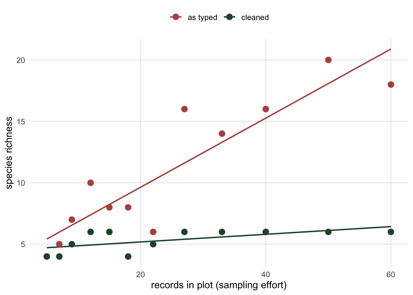
Each extra record adds about `r round(coef(fit)[2], 2)` of a spurious species, and the effect is strong: the p-value in the output above is well under 0.001 on twelve plots. The damage is in the last two numbers. Apparent richness correlates with sampling effort at `r round(cor(per$records, per$apparent), 2)`; true richness correlates at `r round(cor(per$records, per$true), 2)`. The typos have made the effort gradient in richness far steeper than the one in the true names, which only reflects more records finding more of the six species, and effort is rarely random across plots. If the large plots are the productive ones, the misspellings hand you a much stronger productivity to diversity relationship for free, and the extra strength is an artefact of the keyboard.
```{r fig-effort}
#| fig-cap: "Apparent richness, from the names as typed, against sampling effort, with true richness for comparison. The apparent count climbs with effort far faster than the true count, which rises only gently as more records find more of the six species. The extra steepness is a typo gradient, and it will survive into any model that does not clean the names first."
#| fig-alt: "A scatter plot with sampling effort on the horizontal axis. Red points for apparent richness rise steeply from four to twenty as effort increases. Green points for true richness rise only from four to six and then flatten. Two fitted lines make the diverging slopes clear."
long <- rbind(
  data.frame(records = per$records, richness = per$apparent, count = "as typed"),
  data.frame(records = per$records, richness = per$true, count = "cleaned")
)

ggplot(long, aes(records, richness, colour = count)) +
  geom_smooth(method = "lm", formula = y ~ x, se = FALSE, linewidth = 0.8) +
  geom_point(size = 3) +
  scale_colour_manual(values = c("as typed" = "#b5534e", "cleaned" = "#275139")) +
  labs(x = "records in plot (sampling effort)", y = "species richness", colour = NULL) +
  theme_minimal(base_size = 12) + te_canvas +
  theme(legend.position = "top", panel.grid.minor = element_blank())
```
## The trap: fuzzy matching
Writing a lookup table by hand feels like work, and the obvious escape is to let the computer decide which strings are close enough. R measures string distance with `adist`, the number of single character edits between two strings.
```{r adist-typo}
adist("festuca rubra", "fetsuca rubra")
```
Two edits for a transposed pair of letters. So match anything within a distance of two to the nearest accepted name and the typos collapse on their own. The problem arrives when two of the accepted names are themselves close:
```{r adist-real}
adist("carex flacca", "carex flava")
```
Also two. *Carex flacca* and *Carex flava* are two different sedges, and they sit at the same edit distance as a typo and its correct spelling. Any threshold loose enough to fix *fetsuca* is loose enough to merge them, and there is no threshold that separates the real pair from the mistakes.
Here is what that costs when it happens quietly. Suppose last year's reference list is used to snap this year's names, and last year *Carex flava* was never recorded, so it is not on the list.
```{r fuzzy-fail}
reference <- setdiff(tolower(pool), "carex flava")

snap <- function(s, ref, max_edit = 2) {
  d <- adist(s, ref)
  i <- which.min(d)
  if (d[i] <= max_edit) ref[i] else NA_character_
}
matched <- vapply(clean, snap, character(1), ref = reference)

flava_records <- sum(nb$true_name == "Carex flava")
flava_to_flacca <- sum(nb$true_name == "Carex flava" & matched %in% "carex flacca")
c(flava_records = flava_records, silently_relabelled = flava_to_flacca,
  richness_after = length(unique(na.omit(matched))))
```
Most *Carex flava* records fall within two edits of *carex flacca*, so `r flava_to_flacca` of the `r flava_records` get relabelled to it; the rest fail to match anything, and either way the species vanishes from the dataset. Richness drops to `r length(unique(na.omit(matched)))`. Worse, the abundance of the wrong sedge is now inflated:
```{r fuzzy-abundance}
before <- sum(nb$true_name == "Carex flacca")
after <- sum(matched == "carex flacca", na.rm = TRUE)
c(flacca_before = before, flacca_after = after,
  per_cent_change = round(100 * (after / before - 1)))
```
The count for *Carex flacca* rises `r round(100 * (after / before - 1))` per cent, built entirely from another species' records, and nothing in the output flags it. A hand lookup would have hit the missing name and stopped: there is no row for *carex flava*, so it demands a decision instead of guessing. Fuzzy matching guesses, and the guess is silent.
Fuzzy matching has a place as a way to draft the lookup table, listing near matches for a human to confirm. It has no place applying itself unseen, because the one case it cannot handle, two real names a few letters apart, is common in exactly the genera where careful identification matters most.
## What to carry to the next dataset
Richness and every diversity index built on it inherit the spelling of the names, so the names come first, before `unique`, before `diversity`, before any count. The workable order is `trimws`, then collapse internal whitespace, then `tolower`, and then a lookup table for everything that is left, kept as a file. Read the plateau on the funnel figure as the honest signal: when string cleaning stops removing names well above your known species total, the rest is identity, not layout, and it is a decision to be written down rather than a function to be called.
## Where to go next
The cleaned names feed straight into [Diversity indices in R](../diversity-indices-in-r/) and [Rarefaction and accumulation curves](../rarefaction-accumulation-curves/), which is the honest way to compare richness across the uneven effort this post exposed. The lookup step is a join, covered in [Reading field data into R](../reading-field-data-into-r/).
## References
- Wickham H 2014 Journal of Statistical Software 59(10):1-23 (10.18637/jss.v059.i10)
- Boakes EH, Gliozzo G, Seymour V, Harvey M, Smith C, Roy DB, Haklay M 2016 Scientific Reports 6:33051 (10.1038/srep33051)
- Chao A, Gotelli NJ, Hsieh TC, Sander EL, Ma KH, Colwell RK, Ellison AM 2014 Ecological Monographs 84(1):45-67 (10.1890/13-0133.1)
## Related tutorials
- [Recoding field data in R: ifelse, if_else, case_when](../recoding-with-case-when/)
- [Taxonomic revision and species trends](../taxonomic-revision-and-species-trends/)
- [Diversity indices in R](../diversity-indices-in-r/)
- [Text and regular expressions in R](../text-and-regular-expressions/)