---
title: "Wide and long: reshaping species data"
description: "Move a species table between wide and long shape with pivot_longer, pivot_wider and xtabs, and see what a field notebook loses because it cannot write a zero."
date: "2026-06-18 11:00"
date-modified: "2026-10-14"
categories: [R, data import, community ecology, ecology tutorial, tidyr]
image: thumbnail.png
image-alt: "Diagram of the same six counts in two table shapes: a compact wide grid of plots by species, and a taller long table with one row per observation."
---
*Corrected 14 October 2026: the closing rule said that a row count different from quadrats times species shows either your zeros or your duplicates; it now says to count the rows for each quadrat and species pair, because in the total the two can cancel. The post also said that no rule gives the right count for a line typed in twice, where `mean` and `max` do, and that the faceted figure comes from Your first ggplot, which draws one quadrat's counts; it now says that post starts from the long shape and explains the pieces of the figure.*
*Corrected 1 October 2026: the post said that `pivot_wider` stops on a duplicated row and that `diversity()` would have to average a column of quadrat names; it now says that `pivot_wider` warns and returns a list column, and that `diversity()` would have to do arithmetic on the names.*
The same thirty numbers can sit in a table two ways, and R has firm opinions about which. `vegan` will not take the long one. `ggplot2` will take the wide one only one column at a time. Neither shape is the correct one; they are two encodings of the same counts, and one function call moves between them in each direction.
The move is free in only one direction. Going the other way, a field notebook in the long shape cannot say the word zero, and it cannot say which of two rows for the same quadrat you meant.
## Two shapes, thirty numbers
```{r shapes}
wide <- data.frame(
  plot      = paste0("P", 1:6),
  Festuca   = c(42, 38, 51, 63, 29, 44),
  Trifolium = c(7, 0, 2, 5, 9, 4),
  Plantago  = c(3, 4, 1, 6, 7, 2),
  Achillea  = c(5, 6, 0, 4, 3, 8),
  Bromus    = c(11, 9, 14, 12, 0, 10)
)
wide
```
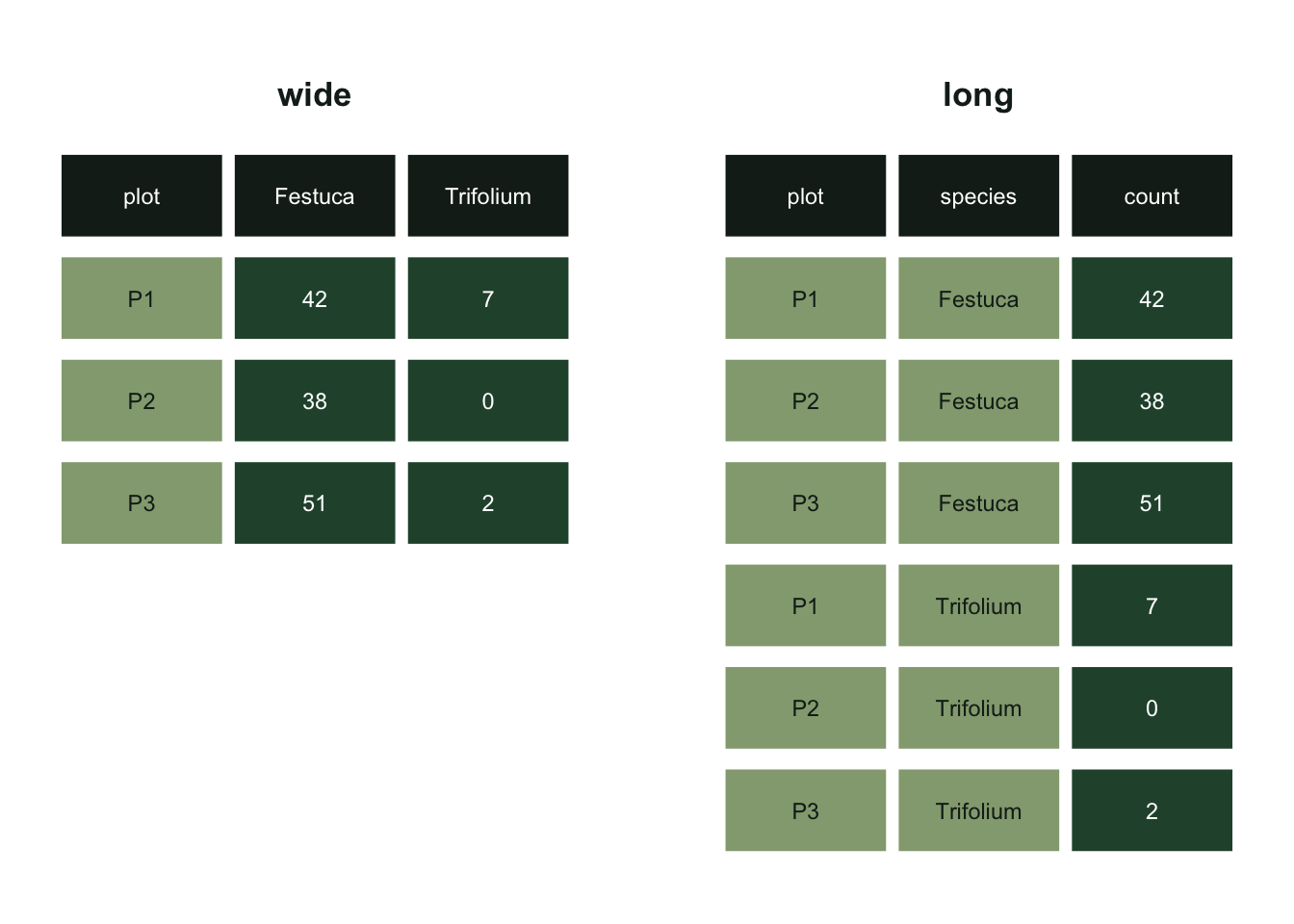
This is the wide shape, and it is what a field sheet looks like: one row per quadrat, one column per species, a count in the cell. It is also called a community matrix or a sites by species matrix, and every multivariate method in ecology expects it.
The long shape says the same thing with one row per observation.
```{r long}
library(tidyr)

long <- pivot_longer(wide, cols = -plot, names_to = "species", values_to = "count")
head(long, 4)
dim(long)
```
Thirty rows of three columns instead of six rows of six. The counts are the same counts. What changed is that the species name has moved out of the column heading and into a cell of its own, which is the whole difference between the two shapes: in the wide table the species is part of the structure, in the long table it is data.
```{r fig-shapes}
#| fig-cap: "A corner of the table, six counts, drawn in both shapes. Green cells hold the counts and sage cells hold the labels that say which quadrat and which species. In the wide table the species name is a column heading; in the long table it has become a column of its own, so every count carries its own labels."
#| fig-alt: "Two tables drawn as grids of coloured cells. On the left a wide table of three quadrat rows with columns for Festuca and Trifolium. On the right a long table of six rows, each carrying a plot label, a species name and one count. Both hold the same six green count cells."
library(ggplot2)
te_canvas <- theme(plot.background  = element_rect(fill = "#f5f4ee", colour = NA),
                   panel.background = element_rect(fill = "#f5f4ee", colour = NA))

cell <- function(x, y, lab, kind) data.frame(x = x, y = y, lab = lab, kind = kind)
w_tab <- rbind(
  cell(c(1, 2.2, 3.4), 7, c("plot", "Festuca", "Trifolium"), "head"),
  cell(rep(1, 3), 6:4, c("P1", "P2", "P3"), "key"),
  cell(rep(2.2, 3), 6:4, c("42", "38", "51"), "value"),
  cell(rep(3.4, 3), 6:4, c("7", "0", "2"), "value")
)
l_tab <- rbind(
  cell(c(5.6, 6.8, 8), 7, c("plot", "species", "count"), "head"),
  cell(rep(5.6, 6), 6:1, rep(c("P1", "P2", "P3"), 2), "key"),
  cell(rep(6.8, 6), 6:1, rep(c("Festuca", "Trifolium"), each = 3), "key"),
  cell(rep(8, 6), 6:1, c("42", "38", "51", "7", "0", "2"), "value")
)
tabs <- rbind(w_tab, l_tab)

ggplot(tabs, aes(x, y, fill = kind)) +
  geom_tile(width = 1.15, height = 0.85, colour = "white", linewidth = 1) +
  geom_text(aes(label = lab, colour = kind), size = 3.1) +
  annotate("text", x = 2.2, y = 8, label = "wide", fontface = "bold",
           colour = "#16241d", size = 4.6) +
  annotate("text", x = 6.8, y = 8, label = "long", fontface = "bold",
           colour = "#16241d", size = 4.6) +
  scale_fill_manual(values = c(head = "#16241d", key = "#93a87f", value = "#275139")) +
  scale_colour_manual(values = c(head = "white", key = "#16241d", value = "white")) +
  scale_y_continuous(limits = c(0.3, 8.5)) +
  guides(fill = "none", colour = "none") +
  theme_void() + te_canvas
```
## The round trip is exact
```{r roundtrip}
back <- pivot_wider(long, names_from = species, values_from = count)
identical(as.data.frame(back), wide)
```
`pivot_longer` and `pivot_wider` are inverses on a complete table, and the check above is worth running once so that you believe it. Nothing is lost, nothing is rounded, and the shape is a presentation choice rather than a decision about the data.
That is true for this table because every quadrat by species combination has a row, including the three that are zero. Hold on to that condition; the rest of the post is about what happens when it fails.
## What each shape is for
`vegan` wants the wide matrix, and it wants it as a matrix of numbers with the quadrat names attached as row names rather than as a column.
```{r vegan-way}
suppressPackageStartupMessages(library(vegan))

m <- as.matrix(wide[, -1])
rownames(m) <- wide$plot
round(diversity(m), 3)
```
Leave the quadrat column in and the error is immediate, and worth recognising because everyone meets it:
```{r vegan-trap}
try(diversity(wide))
```
`diversity()` is not being fussy. It would have to do arithmetic on a column of quadrat names, so it stops. The two lines that fix it are the `as.matrix(wide[, -1])` and the `rownames()` above, and they are the standard preamble to every `vegan` call in this blog.
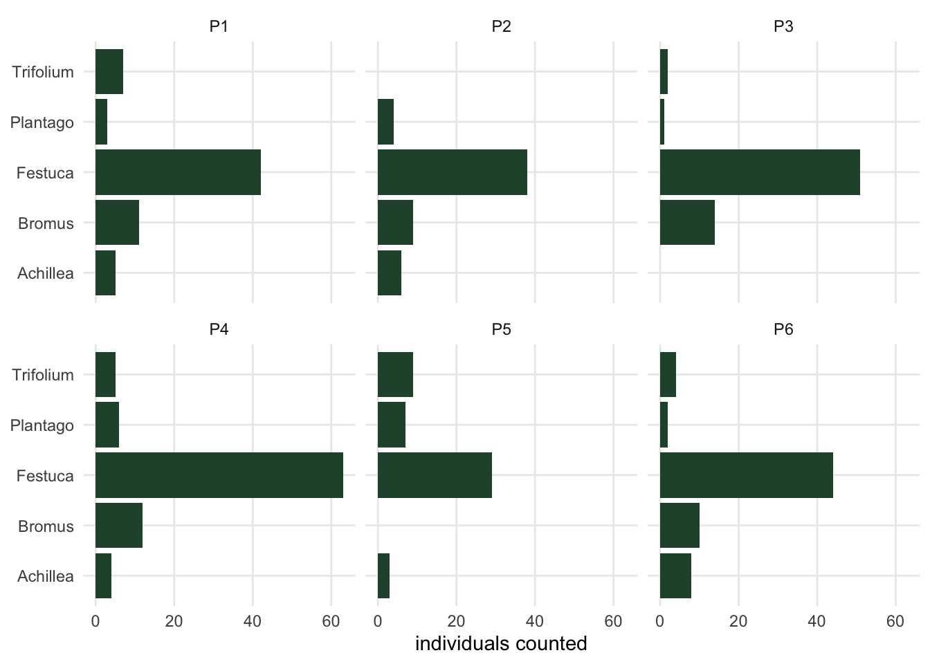
`ggplot2` wants the opposite. It maps columns to axes, colours and panels, so anything you want on an axis has to be a column, and in the wide table the species is not a column.
```{r fig-long-plot}
#| fig-cap: "The long table plotted directly: one panel per quadrat, one bar per species. The species name can go on an axis because it is a column. The same figure from the wide table would need five separate calls, one per species column."
#| fig-alt: "Six small panels, one for each quadrat, each showing five horizontal bars for Festuca, Trifolium, Plantago, Achillea and Bromus. Festuca is much the longest bar in every panel. Trifolium is absent from P2, Achillea from P3 and Bromus from P5."
ggplot(long, aes(x = count, y = species)) +
  geom_col(fill = "#275139") +
  facet_wrap(~plot) +
  labs(x = "individuals counted", y = NULL) +
  theme_minimal(base_size = 11) + te_canvas +
  theme(panel.grid.minor = element_blank())
```
Five species, one call. From the wide table the same figure needs one call per species column, and the code grows every time a species is added. This is the practical reason the long shape exists, and it is the whole of the reason: it is not tidier in any moral sense, it is just the shape whose columns match what a plot needs.
## The notebook that cannot write a zero
Field notebooks are already long, and that is the good news. The bad news is that a notebook only has rows for what somebody saw.
```{r notebook}
notebook <- subset(long, count > 0)
c(notebook_rows = nrow(notebook), full_grid = nrow(long))
```
`r nrow(long) - nrow(notebook)` rows are missing, and they are exactly the zeros: nobody writes a line in a notebook to record that Trifolium was not in P2. Now pivot it back.
```{r notebook-wide}
nb <- pivot_wider(notebook, names_from = species, values_from = count)
m_nb <- as.matrix(nb[, -1])
rownames(m_nb) <- nb$plot
m_nb
```
`pivot_wider` had to put something in the cells with no row, and what it puts there is `NA`. This is the correct default: the function was handed a table with no line for Trifolium in P2, and inventing a zero would be a claim about the field that nothing in the file supports. The consequence is the one from [Reading field data into R](../reading-field-data-into-r/):
```{r notebook-diversity}
round(diversity(m_nb), 3)
```
`r sum(is.na(diversity(m_nb)))` of the `r nrow(m_nb)` quadrats come back as `NA`, from a notebook where nothing was missing at all. The `values_fill` argument is where you say what the gaps mean.
```{r notebook-fill}
nb0 <- pivot_wider(notebook, names_from = species, values_from = count, values_fill = 0)
m_fill <- as.matrix(nb0[, -1])
rownames(m_fill) <- nb0$plot
m_fill <- m_fill[rownames(m), colnames(m)]
max(abs(m_fill - m))
```
The table is exactly the one we started with. `values_fill = 0` is the right call here, and the reason it is right has nothing to do with R: this notebook records every species the recorder looked for, so a species with no line was looked for and not found. If the notebook only lists what was interesting that day, the same argument fails and the same zero is a fabrication.
Base R does the whole thing in one line, and it fills the zeros without being asked:
```{r xtabs}
xt <- xtabs(count ~ plot + species, data = notebook)
identical(as.numeric(xt[rownames(m), colnames(m)]), as.numeric(m))
```
`xtabs` builds a contingency table, and an absent combination in a contingency table is a count of zero by definition, so the fill is baked in. It returns a table rather than a data frame, which `vegan` accepts, and it needs no packages. The formula reads: `count`, broken down by `plot` and `species`.
## Two rows, one cell
Here is the failure that is worth the price of this post. Somebody counted Festuca in P1 twice, in two subplots, and wrote two lines.
```{r dup}
dup <- rbind(as.data.frame(notebook),
             data.frame(plot = "P1", species = "Festuca", count = 8))
subset(dup, plot == "P1" & species == "Festuca")
```
There is now one cell in the wide table with two candidate values. `pivot_wider` refuses to choose.
```{r dup-pivot}
#| warning: true
res <- pivot_wider(dup, names_from = species, values_from = count)
class(res$Festuca)
res$Festuca[[1]]
```
The warning is the important output. The column is now a list, each entry holding every value that landed in that cell, and any analysis downstream fails on it. Ask for the fill as well and the refusal turns into an error, because a list column and a fill value of zero cannot both be true.
```{r dup-error}
try(pivot_wider(dup, names_from = species, values_from = count, values_fill = 0))
```
Now the same data through `xtabs`:
```{r dup-xtabs}
xd <- xtabs(count ~ plot + species, data = dup)
xd["P1", "Festuca"]
```
No warning, no error, one number. `xtabs` sums, because summing is what a contingency table does, and the sum is a defensible answer here. It is not the only defensible answer.
```{r dup-rules}
rules <- list(sum = sum, mean = mean, max = max)
out <- sapply(rules, function(f) {
  w <- suppressWarnings(pivot_wider(dup, names_from = species,
                                    values_from = count, values_fn = f))
  mm <- as.matrix(w[, -1])
  rownames(mm) <- w$plot
  mm <- mm[rownames(m), colnames(m)]
  c(P1_Festuca = unname(mm["P1", "Festuca"]), P1_Shannon = diversity(mm["P1", ]))
})
round(out, 4)
```
Three rules, three numbers, and each is right for a different field design. If the two lines are two subplots of the same quadrat, the quadrat total is `r out["P1_Festuca", "sum"]` and `sum` is correct. If they are two visits to the same quadrat, the sum counts many of the same plants twice and `max` or `mean` is closer. If somebody typed the line in twice, the two rows carry the same count, so `mean` and `max` return it while `sum` doubles it, and one row should go. The counts do not know which, and neither does the function.
It matters at the scale of the study, not just of the cell.
```{r dup-scale}
delta <- unname(out["P1_Shannon", "sum"] - out["P1_Shannon", "mean"])
pairs <- as.numeric(dist(diversity(m)))
c(rule_effect = round(abs(delta), 4),
  smaller_pairs = sum(pairs < abs(delta)),
  total_pairs = length(pairs),
  study_range = round(diff(range(diversity(m))), 4))
```
Choosing `mean` over `sum` for one duplicated line moves the Shannon index of P1 by `r round(abs(delta), 3)`. That is larger than `r sum(pairs < abs(delta))` of the `r length(pairs)` differences between pairs of quadrats in this study, and it is `r round(100 * abs(delta) / diff(range(diversity(m))))` per cent of the range across all six. `xtabs` picks one of the three rules silently, and that is the argument for the noisier function: `pivot_wider` warns, hands back a list column that no analysis will take, and so makes you write down which design you had.
## The honest limit
Reshaping is arithmetic and it is exact, in both directions, as long as the table is complete. Everything difficult in this post happened at the boundary where the table stops being complete: the missing zero and the doubled row. Neither is a reshaping problem. Both are questions about the field protocol that arrive disguised as an argument to a function, and `values_fill` and `values_fn` are the two places R asks you to answer them.
The rule that survives: with the data in the long shape, count the rows for every quadrat and species pair, for example with `table(dup$plot, dup$species)`. A pair with no row is a gap and a pair with more than one row is a duplicate, and you should know what each one means before the analysis starts. The total alone is not enough: `nrow(long)` equals quadrats times species when the grid is complete, but gaps lower it and duplicates raise it, so the two can cancel.
## Where to go next
The wide matrix built here is the input to [Diversity indices in R](../diversity-indices-in-r/) and to every ordination on this site. The long shape is the one [Your first ggplot: data, aes and geom](../your-first-ggplot/) starts from, and that post explains the data, aes and geom behind the figure above.
## References
- Wickham H 2014 Journal of Statistical Software 59(10):1-23 (10.18637/jss.v059.i10)
- Broman KW, Woo KH 2018 The American Statistician 72(1):2-10 (10.1080/00031305.2017.1375989)
- Borcard D, Gillet F, Legendre P 2018 Numerical Ecology with R, 2nd edn, Springer (ISBN 978-3-319-71403-5)
## Related tutorials
- [Reading field data into R](../reading-field-data-into-r/)
- [Your first ggplot: data, aes and geom](../your-first-ggplot/)
- [Cleaning species names before you count](../cleaning-species-names/)
- [Diversity indices in R](../diversity-indices-in-r/)