sheet_lines <- c(
  "plot,Festuca,Trifolium,Plantago,Achillea,Bromus,notes",
  "P1,42,7,3,5,11,",
  "P2,38,,4,6,9,",
  "P3,51,2,1,,14,",
  "P4,n/a,5,6,4,12,no time for the grass",
  "P5,29,9,7,3,,",
  "P6,44,4,2,8,10,"
)
csv_path <- file.path(tempdir(), "quadrats.csv")
writeLines(sheet_lines, csv_path)Reading field data into R
R
data import
missing data
ecology tutorial
vegan
Read a field spreadsheet into R with read.csv, see why empty cells arrive as NA, and measure what replacing every NA with a zero does to a Shannon index.
Step 2 of the Tidy Ecology course, Part one: get the data into R.
Corrected 15 October 2026: the gap map’s caption said nothing in the file tells the zeros from the uncounted cell; the file marks that cell with a typed n/a and a note, and the caption now says it is read.csv that gives all four the same NA. The post also said the four gaps carry three field histories; they carry two of the three a gap can have.
Corrected 27 September 2026: the Shannon figure labelled the true counts as the values recorded in the field; the legend and caption now call them the true counts.
Updated 27 September 2026: a new section, Arithmetic fails loudly, comparisons do not, shows what a count column read as text does to a filter such as Festuca > 5, which returns the wrong quadrats without a warning.
The first thing most ecologists do in R is read a spreadsheet, and it is the step where most first sessions stall. The counts are on the clipboard, the clipboard becomes a CSV, and then R says something about an invalid type of argument.
This post takes one small quadrat sheet from the file to a Shannon index, and stops at each point where R quietly does something you did not ask for. By the end, the quadrat with the missing count is the most diverse quadrat in the study, and nothing on the way there produces a warning.
The sheet
Six quadrats, five species, counts of individuals. Rather than ask you to download anything, the code writes the sheet to a temporary file so that every line below runs as it stands. Your own file would live in a data/ folder inside your project, and the path would read data/quadrats.csv.
Four things about this sheet are entirely ordinary, and all four matter. Three cells are blank. One cell says n/a, because somebody typed it. The notes column is mostly empty. And nowhere on the sheet is there anything that says which of those blanks means zero.
Look at the types before you look at the numbers
naive <- read.csv(csv_path)
str(naive)
'data.frame': 6 obs. of 7 variables:
$ plot : chr "P1" "P2" "P3" "P4" ...
$ Festuca : chr "42" "38" "51" "n/a" ...
$ Trifolium: int 7 NA 2 5 9 4
$ Plantago : int 3 4 1 6 7 2
$ Achillea : int 5 6 NA 4 3 8
$ Bromus : int 11 9 14 12 NA 10
$ notes : chr "" "" "" "no time for the grass" ...str() is the line to run after every read.csv, and it answers one question: what type is each column? Here the answer is a problem.
class(naive$Festuca)[1] "character"Festuca came in as character. One cell out of thirty was typed as n/a, and R applied its only rule for a column: every value has the same type, so if one of them cannot be a number, none of them are. The column of counts is now a column of words, and arithmetic on it fails.
try(sum(naive$Festuca))Error in sum(naive$Festuca) : invalid 'type' (character) of argumentThat error message is the single most common way a first R script dies, and it names the symptom rather than the cause. The cause is three characters in one cell.
Arithmetic fails loudly, comparisons do not
The error is the helpful case. Arithmetic on a text column stops, or at least complains.
try(naive$Festuca * 2)Error in naive$Festuca * 2 : non-numeric argument to binary operatortryCatch(mean(naive$Festuca), warning = conditionMessage)[1] "argument is not numeric or logical: returning NA"tryCatch(as.numeric(naive$Festuca), warning = conditionMessage)[1] "NAs introduced by coercion"Multiplication stops with an error. mean() does not stop: it warns and returns NA. as.numeric() also warns, once, that it turned something into NA. (The tryCatch() lines print the text of each warning in place of the result, so you can read it here.) A laboratory export that writes each non-detect as <0.1 fails in the same way, and Values below the detection limit in R shows why stripping the < is not the cure.
A comparison is different. Which quadrats have more than five Festuca is a question about numbers, and R answers it on the text without a word.
fest_num <- suppressWarnings(as.numeric(naive$Festuca))
data.frame(plot = naive$plot, as_read = naive$Festuca,
           text_over_5 = naive$Festuca > 5, count_over_5 = fest_num > 5,
           text_over_40 = naive$Festuca > 40, count_over_40 = fest_num > 40)
plot as_read text_over_5 count_over_5 text_over_40 count_over_40
1 P1 42 FALSE TRUE TRUE TRUE
2 P2 38 FALSE TRUE FALSE FALSE
3 P3 51 TRUE TRUE TRUE TRUE
4 P4 n/a TRUE NA TRUE NA
5 P5 29 FALSE TRUE FALSE FALSE
6 P6 44 FALSE TRUE TRUE TRUEnaive$plot[naive$Festuca > 5][1] "P3" "P4"max(naive$Festuca)[1] "n/a"stopifnot(identical(naive$plot[naive$Festuca > 5], c("P3", "P4")),
identical(naive$plot[naive$Festuca > 40], c("P1", "P3", "P4", "P6")),
identical(max(naive$Festuca), "n/a"),
sum((naive$Festuca > 40) != (fest_num > 40), na.rm = TRUE) == 0,
all(nchar(naive$Festuca[!is.na(fest_num)]) == 2),
!("100" > 40))When one side of > is text, R turns the other side into text as well, so 5 becomes "5", and the two are compared the way a dictionary orders words: one character at a time from the left. "42" against "5" is settled by "4" against "5", so 42 is not more than 5. Of the 5 counted quadrats with more than five Festuca, the filter keeps 1 (P3), and it adds P4, where nobody counted the grass, because here letters sort after digits. At 40 the text gets every counted quadrat right, because every count here has two digits, like 40, and then text order and number order agree; only the n/a slips in. One count of 100 would break it again, since "100" sorts before "40". A filter that looks right at one threshold, on one sheet, says nothing about the next. max() returns "n/a" as the largest count. None of the comparisons, and not max(), printed a warning.
This is the same dictionary order that turns a factor of numbers into the wrong codes, which Debugging and defensive R code takes apart. Text comparison follows the sorting rules of the language your computer is set to (the help page ?Comparison says so), which is why the chunk checks its own answer with stopifnot(). The rule is the one str() already taught: a column that should hold numbers is fixed when the file is read, never compared as it stands. That fix is the next section.
Tell read.csv what missing looks like
read.csv treats an empty field as missing in a numeric column and as an empty string in a text column, and it has never heard of n/a. The na.strings argument is where you declare your conventions.
sheet <- read.csv(csv_path, na.strings = c("", "n/a", "NA"))
str(sheet)
'data.frame': 6 obs. of 7 variables:
$ plot : chr "P1" "P2" "P3" "P4" ...
$ Festuca : int 42 38 51 NA 29 44
$ Trifolium: int 7 NA 2 5 9 4
$ Plantago : int 3 4 1 6 7 2
$ Achillea : int 5 6 NA 4 3 8
$ Bromus : int 11 9 14 12 NA 10
$ notes : chr NA NA NA "no time for the grass" ...colSums(is.na(sheet)) plot Festuca Trifolium Plantago Achillea Bromus notes
0 1 1 0 1 1 5 The counts are integers again. Note what happened in the notes column: before the fix, is.na(naive$notes) found 0 missing notes, while naive$notes == "" found 5. A blank cell in a text column arrives as an empty string, and an empty string is not missing as far as R is concerned. It is the same fix, and it is the reason na.strings includes "".
One blank, three meanings
There are 4 missing counts on this sheet. Gaps like these can carry three different field histories.
- The species was looked for and was not there. The count is zero, and the recorder left the cell empty because writing zeros is boring.
- The species was not counted. On P4 the grass was left for later and later never came. The count exists in the quadrat; it is simply not on the sheet.
- Somebody skipped a cell by mistake, and nobody knows which case it was.
R receives one thing for all three: NA. This is not a flaw in read.csv. The information was not written down, so it is not in the file, and no argument to any function can bring it back.
What NA costs you
suppressPackageStartupMessages(library(vegan))

m <- as.matrix(sheet[, 2:6])
rownames(m) <- sheet$plot
round(diversity(m), 3)
P1 P2 P3 P4 P5 P6
1.156 NA NA NA NA 1.086 diversity() does not guess. One NA anywhere in a row and the Shannon index for that row is NA, so 4 of the 6 quadrats came back empty, from four missing counts out of thirty: the three blank cells and the one that said n/a. This is the well behaved outcome: the function refuses rather than inventing.
Replacing NA with zero is a claim about the field
The reflex at this point is to write zeros over the gaps.
m0 <- m
m0[is.na(m0)] <- 0
round(diversity(m0), 3)
P1 P2 P3 P4 P5 P6
1.156 0.985 0.707 1.290 1.072 1.086 Six numbers, no warnings. Before using them, it is worth being precise about what a zero does to a Shannon index. Shannon sums -p * log(p) over the species that are present, and a species with zero individuals contributes nothing and adds nothing to the total either. So a zero and a species that was never on the sheet give the same number, exactly:
p4_zero <- m0["P4", ]
p4_drop <- p4_zero[p4_zero > 0]
c(with_zero = diversity(p4_zero), species_dropped = diversity(p4_drop))
with_zero species_dropped
1.289844 1.289844 diversity(p4_zero) - diversity(p4_drop)[1] 0The two are not close, they are the same number, and the gap between them is 0. Writing a zero into a cell is arithmetically identical to deleting the species from that quadrat. It is a statement that the species was looked for and was not found.
For three of these gaps the statement is true, and this is the case worth remembering, because filling them in costs nothing at all. Since this sheet is an invented example, we can write down what the recorder would have counted:
truth <- data.frame(
  plot      = paste0("P", 1:6),
  Festuca   = c(42, 38, 51, 63, 29, 44),
  Trifolium = c(7, 0, 2, 5, 9, 4),
  Plantago  = c(3, 4, 1, 6, 7, 2),
  Achillea  = c(5, 6, 0, 4, 3, 8),
  Bromus    = c(11, 9, 14, 12, 0, 10)
)
m_true <- as.matrix(truth[, -1])
rownames(m_true) <- truth$plot
H_true <- diversity(m_true)
H_zero <- diversity(m0)

round(cbind(truth = H_true, filled = H_zero, difference = H_zero - H_true), 4)
truth filled difference
P1 1.1559 1.1559 0.000
P2 0.9852 0.9852 0.000
P3 0.7069 0.7069 0.000
P4 0.9978 1.2898 0.292
P5 1.0724 1.0724 0.000
P6 1.0857 1.0857 0.000P2, P3 and P5 are exact. Their blanks were genuine absences, the zero says so, and the Shannon index is untouched. P4 is not exact, because on P4 the gap meant that nobody counted the Festuca, and there were 63 of them.
c(true_H = unname(H_true["P4"]), filled_H = unname(H_zero["P4"])) true_H filled_H
0.9978175 1.2898441 round(unname(100 * (H_zero["P4"] / H_true["P4"] - 1)), 1)[1] 29.3c(true_richness = sum(m_true["P4", ] > 0), filled_richness = sum(m0["P4", ] > 0)) true_richness filled_richness
5 4 The Shannon index for P4 is 29.3 per cent too high, and the direction is the part to sit with. The quadrat lost its dominant species, and a community without its dominant looks more even, not less. The error made the quadrat look better, not broken.
rank_true <- names(sort(H_true, decreasing = TRUE))
rank_zero <- names(sort(H_zero, decreasing = TRUE))
rbind(truth = rank_true, filled = rank_zero)
[,1] [,2] [,3] [,4] [,5] [,6]
truth "P1" "P6" "P5" "P4" "P2" "P3"
filled "P4" "P1" "P6" "P5" "P2" "P3"P4 is the fourth most diverse quadrat of six. After the zero it is the first. If those six numbers went into a figure, or into a test against a management treatment, nothing in the output would point back at one empty cell.
library(ggplot2)
te_canvas <- theme(plot.background  = element_rect(fill = "#f5f4ee", colour = NA),
                   panel.background = element_rect(fill = "#f5f4ee", colour = NA))

cmp <- rbind(
  data.frame(plot = names(H_true), H = as.numeric(H_true), source = "true counts"),
  data.frame(plot = names(H_zero), H = as.numeric(H_zero), source = "blanks filled with zero")
)
gap <- data.frame(plot = names(H_true), lo = as.numeric(H_true), hi = as.numeric(H_zero))

ggplot(cmp, aes(plot, H)) +
  geom_segment(data = gap, aes(x = plot, xend = plot, y = lo, yend = hi),
               inherit.aes = FALSE, colour = "#dad9ca", linewidth = 1.2) +
  geom_point(aes(colour = source, shape = source), size = 3.4) +
  scale_colour_manual(values = c("true counts" = "#275139",
                                 "blanks filled with zero" = "#b5534e"),
                      breaks = c("true counts", "blanks filled with zero")) +
  scale_shape_manual(values = c("true counts" = 16, "blanks filled with zero" = 17),
                     breaks = c("true counts", "blanks filled with zero")) +
  labs(x = NULL, y = "Shannon index", colour = NULL, shape = NULL) +
  theme_minimal(base_size = 12) + te_canvas +
  theme(legend.position = "top", panel.grid.minor = element_blank())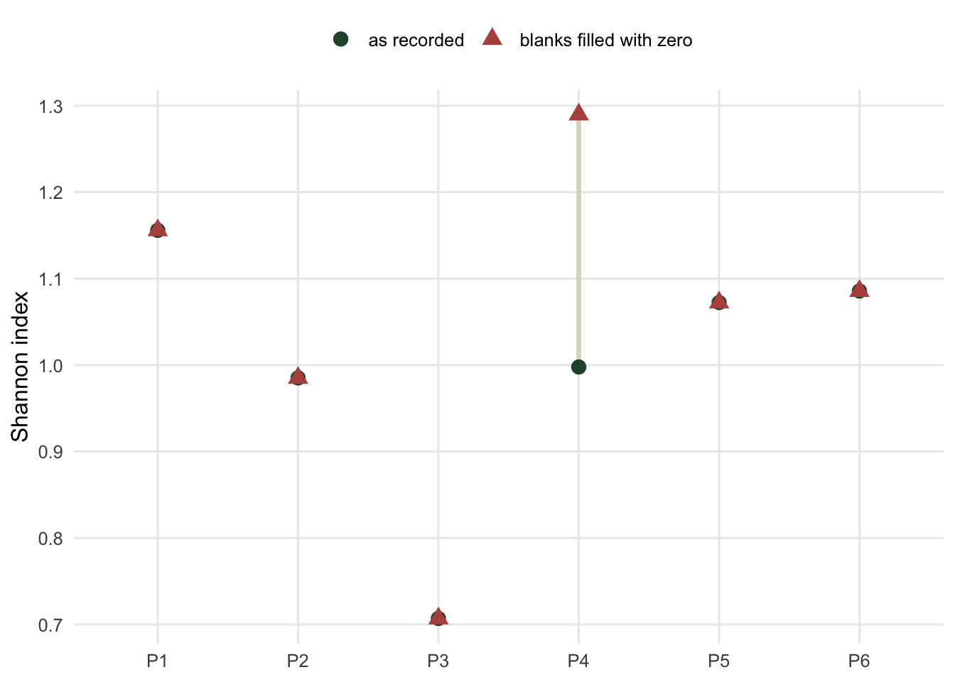
The repair is on the clipboard, not in R
Everything above followed from a sheet that cannot distinguish an absence from an omission. That is a recording problem, and it has a recording solution: write the zeros, and give the gaps a code of their own.
good_lines <- c(
  "plot,Festuca,Trifolium,Plantago,Achillea,Bromus",
  "P1,42,7,3,5,11",
  "P2,38,0,4,6,9",
  "P3,51,2,1,0,14",
  "P4,NS,5,6,4,12",
  "P5,29,9,7,3,0",
  "P6,44,4,2,8,10"
)
good_path <- file.path(tempdir(), "quadrats_ns.csv")
writeLines(good_lines, good_path)

good <- read.csv(good_path, na.strings = "NS")
mg <- as.matrix(good[, -1])
rownames(mg) <- good$plot
H_good <- diversity(mg)
round(H_good, 3)
P1 P2 P3 P4 P5 P6
1.156 0.985 0.707 NA 1.072 1.086 NS for not surveyed, zero for absent, and one argument to read.csv turns the code back into NA. There is now exactly 1 missing value on the sheet, and it is the one that is genuinely missing.
complete <- setdiff(rownames(mg), "P4")
max(abs(H_good[complete] - H_true[complete]))
[1] 0The five complete quadrats reproduce the truth to the last digit, and P4 returns NA, which is the correct answer to the question that was asked. Nobody counted the grass, so nobody knows how diverse P4 was. The sheet that carries the field protocol gives you five honest numbers and one honest refusal; the sheet that hides it gives you six numbers, one of which is wrong in a direction that flatters the study.
Broman and Woo (2018) put this as a rule for spreadsheets: fill in every cell, and use a single agreed code for missing values. White and colleagues (2013) make the same point for ecological data specifically, and both are worth the twenty minutes before your next field season rather than after it.
The check to run every time
Three lines, before any analysis touches the table.
str(sheet)'data.frame': 6 obs. of 7 variables:
$ plot : chr "P1" "P2" "P3" "P4" ...
$ Festuca : int 42 38 51 NA 29 44
$ Trifolium: int 7 NA 2 5 9 4
$ Plantago : int 3 4 1 6 7 2
$ Achillea : int 5 6 NA 4 3 8
$ Bromus : int 11 9 14 12 NA 10
$ notes : chr NA NA NA "no time for the grass" ...colSums(is.na(sheet)) plot Festuca Trifolium Plantago Achillea Bromus notes
0 1 1 0 1 1 5 sapply(sheet[, 2:6], function(x) range(x, na.rm = TRUE)) Festuca Trifolium Plantago Achillea Bromus
[1,] 29 2 1 3 9
[2,] 51 9 7 8 14str() catches the text column that should be numeric. colSums(is.na()) tells you how many gaps there are and where, which is also the number you should be able to explain from your field notes. The ranges catch the decimal comma, the extra zero and the count of 550 that was meant to be 55.
A map of the gaps is quicker to read than a column of totals once the sheet is bigger than this one.
long <- data.frame(
  plot    = rep(sheet$plot, times = 5),
  species = rep(names(sheet)[2:6], each = nrow(sheet)),
  count   = as.vector(as.matrix(sheet[, 2:6]))
)
long$species <- factor(long$species, levels = names(sheet)[2:6])
long$plot <- factor(long$plot, levels = rev(sheet$plot))

ggplot(long, aes(species, plot, fill = count)) +
  geom_tile(colour = "white", linewidth = 1.1) +
  geom_text(aes(label = ifelse(is.na(count), "NA", count)),
            colour = "white", size = 3.6) +
  scale_fill_gradient(low = "#93a87f", high = "#1d5b4e", na.value = "#b5534e") +
  labs(x = NULL, y = NULL, fill = "count") +
  theme_minimal(base_size = 12) + te_canvas +
  theme(panel.grid = element_blank())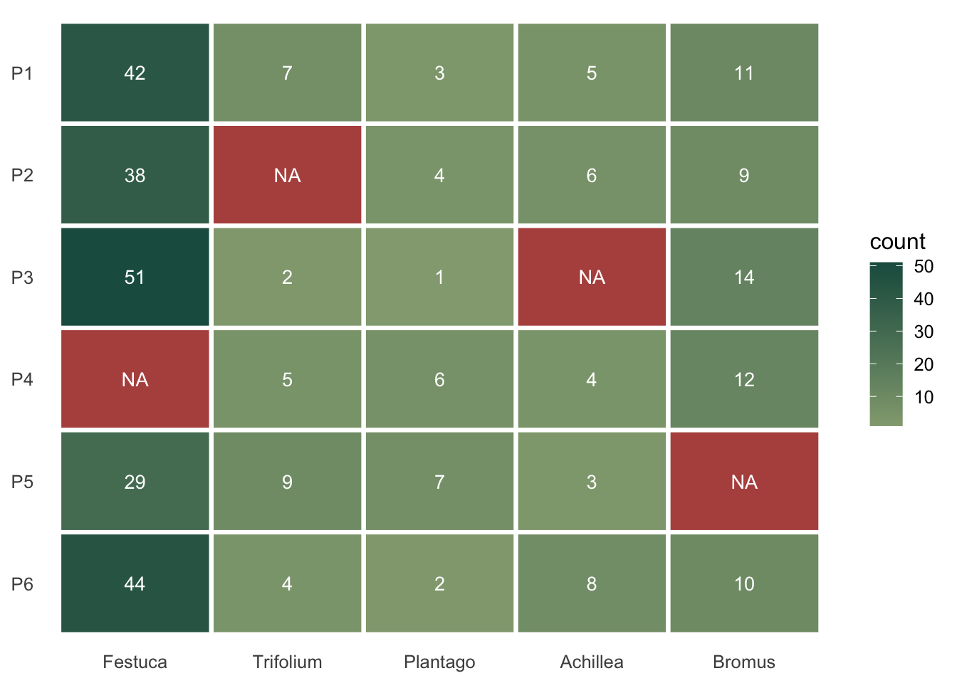
The honest limit
Nothing in R can recover what a blank cell meant. na.strings controls how the file is read, and zero-filling controls what you claim; neither is a measurement. The only place the meaning can exist is the field protocol, and the only place it survives is the sheet itself.
This also puts a boundary on the machinery for missing data. Multiple imputation and its relatives ask what to do when a value that exists was not observed, and they need to know the mechanism. The gap on P4 qualifies. The blanks on P2, P3 and P5 do not, because nothing there is missing at all: the value is zero and the recorder was saving ink. Imputing those would be inventing variation in a cell whose value is known.
Where to go next
With a clean numeric table, the next question is its shape, because vegan and ggplot2 want opposite ones. After that, the analysis in Diversity indices in R runs on a site-by-species matrix like the one built here.
References
- Broman KW, Woo KH 2018 The American Statistician 72(1):2-10 (10.1080/00031305.2017.1375989)
- White EP, Baldridge E, Brym ZT, Locey KJ, McGlinn DJ, Supp SR 2013 Ideas in Ecology and Evolution 6(2):1-10 (10.4033/iee.2013.6b.6.f)
- Zuur AF, Ieno EN, Elphick CS 2010 Methods in Ecology and Evolution 1(1):3-14 (10.1111/j.2041-210X.2009.00001.x)