---
title: "Joining ecological tables without losing zeros"
description: "Joining tables in R with dplyr: why an inner join silently drops the sites where a species was absent and biases abundance, and how a left join keeps the zeros."
date: "2026-06-19 09:00"
date-modified: "2026-09-26"
categories: [R, dplyr, data wrangling, ecology tutorial]
image: thumbnail.png
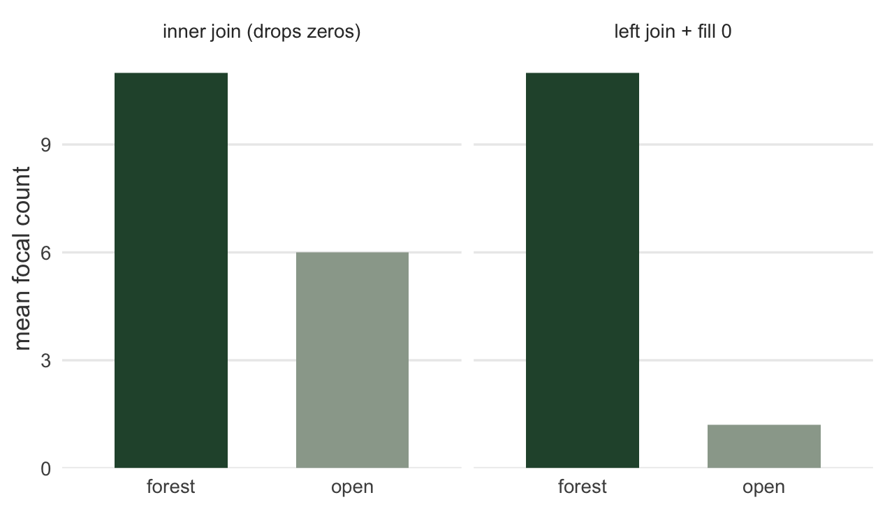
image-alt: "Two bar charts comparing mean focal-species count by habitat under an inner join and a left join, showing the open-habitat bar much higher when zeros are dropped."
---
*Updated 26 September 2026: a new section, A key that appears twice, shows how a site listed twice in one table copies rows in a join, when dplyr warns about it and when it says nothing.*
Field data almost never lives in one table. You keep a **site table** with every site you surveyed and its attributes (habitat, elevation, date), and a separate **observation table** with the counts, one row per species seen. To analyse anything you have to join them, and the default way of joining two tables in R does something that quietly corrupts abundance and occupancy summaries: it throws away the sites where your focal species was never recorded.
This post covers the join verbs in `dplyr` and then shows the measurable damage. The absent sites are real zeros, and dropping them biases mean abundance upward by two thirds and shrinks a genuine habitat effect fivefold.
## The two tables
Here is a survey of ten sites for one focal species. Every site was visited (the survey frame is complete), and each site is either forest or open:
```{r}
#| label: site-table
#| message: false
library(dplyr)
library(tidyr)
sites <- data.frame(
  site    = paste0("S", 1:10),
  habitat = c(rep("forest", 5), rep("open", 5))
)
sites
```
The observation table holds the focal-species counts, but only for the sites where the species was actually recorded. The species was seen at all five forest sites and at one open site; the other four open sites turned up nothing, so they simply have no row here:
```{r}
#| label: obs-table
obs <- data.frame(
  site  = c("S1", "S2", "S3", "S4", "S5", "S6"),
  count = c(  12,    9,   15,    8,   11,    6)
)
obs
```
Those four missing sites are the whole problem. They are not missing data: the species was looked for and not found, so its count there is zero. But a zero count produces no row in a table built from observations, and now the join has to decide what to do with sites that appear in one table and not the other.
## Inner join drops the absent sites
An **inner join** keeps only the sites present in *both* tables. This is what `merge()` does by default and what most people reach for first:
```{r}
#| label: inner
inner <- inner_join(sites, obs, by = "site")
nrow(inner)
```
```{r}
#| label: inner-numbers
#| include: false
mean_inner <- mean(inner$count)
```
Ten surveyed sites became `r nrow(inner)` rows. The four open sites where the species was absent are gone, because they had no row in `obs`. Any summary you now compute is a summary over presence-only sites:
```{r}
#| label: inner-mean
mean(inner$count) # mean over the six sites where the species was seen
```
This mean, `r sprintf("%.2f", mean_inner)`, is not the mean abundance across your survey. It is the mean **given the species was present**, which is a different and almost always larger quantity.
## Left join, then fill the zeros
A **left join** keeps every row of the left table (the survey frame) and attaches the observations where they exist. Sites with no observation get `NA` in the count column, and because we know those `NA` values are true zeros, we replace them:
```{r}
#| label: left
full <- left_join(sites, obs, by = "site") |>
  mutate(count = replace_na(count, 0))
full
```
```{r}
#| label: full-numbers
#| include: false
mean_full <- mean(full$count)
bias <- (mean_inner - mean_full) / mean_full * 100
```
Now all `r nrow(full)` surveyed sites are present, four of them with the zero they earned:
```{r}
#| label: full-mean
mean(full$count) # mean over every surveyed site
```
The mean abundance is `r sprintf("%.2f", mean_full)`, not `r sprintf("%.2f", mean_inner)`. The inner join inflated it by `r sprintf("%.1f", bias)` per cent, purely by deleting zeros.
## A key that appears twice
A join pairs each row of one table with every row of the other table that has the same key, here `site`. If the lookup table (the second table in the join) lists each site once, each row finds at most one partner. If a site appears twice, every row that matches it comes out twice, and each count, mean and sample size after the join includes the copies.
dplyr warns when a row of the left table matches several rows of the lookup table and, somewhere, a row of the lookup table matches several rows of the left table; the two need not be the same site. Suppose every site was visited twice, so a visit table has two rows per site, and the site table was put together from two field sheets that both listed `S7`:
```{r}
#| label: dup-visits
#| warning: true
visits <- data.frame(site  = rep(sites$site, each = 2),
                     visit = rep(1:2, times = 10))
sites_twice <- rbind(sites, sites[sites$site == "S7", ])   # S7 is on both sheets
visits_joined <- left_join(visits, sites_twice, by = "site")
table(visits_joined$habitat)
nrow(merge(visits, sites_twice, by = "site")) # base R: same rows, no warning
```
The `r nrow(visits)` visits became `r nrow(visits_joined)` rows: each of the two `S7` visits matched two rows of the site table, so open habitat counts `r sum(visits_joined$habitat == "open")` visits instead of ten. dplyr (version `r packageVersion("dplyr")` here) calls the left table `x` and the lookup table `y`. It warns because row 13 of `x` (the first `S7` visit) matches two rows of `y`, and row 1 of `y` (`S1`) matches two visits. A visit table repeats every site, so one duplicated site anywhere in the site table is enough to set the warning off. Base `merge()` returns the same rows and says nothing.
The quieter case is when only the lookup table repeats the key. Suppose the count at `S3` was checked against a photograph of the field sheet and should be 5, not 15, and the corrected count was added as a new row at the bottom of `obs` instead of replacing the old one:
```{r}
#| label: dup-appended
obs_appended <- rbind(obs, data.frame(site = "S3", count = 5))   # old S3 row still there
full_appended <- left_join(sites, obs_appended, by = "site") |>
  mutate(count = replace_na(count, 0))
nrow(full_appended)
full_appended |> group_by(habitat) |> summarise(mean_count = mean(count), n_sites = n())
```
```{r}
#| label: dup-guards
#| include: false
said <- function(expr) { # every warning or message an expression gives
out <- character(0)
keep <- function(cnd) { out <<- c(out, conditionMessage(cnd)); tryInvokeRestart("muffleWarning"); tryInvokeRestart("muffleMessage") }
withCallingHandlers(expr, warning = keep, message = keep)
out
}
said_visits <- said(left_join(visits, sites_twice, by = "site"))
obs_corrected <- transform(obs, count = ifelse(site == "S3", 5, count))
forest_mean <- function(tab) { # forest mean count after the left join and zero fill
joined <- left_join(sites, tab, by = "site") |> mutate(count = replace_na(count, 0))
mean(joined$count[joined$habitat == "forest"]) }
error_text <- function(expr) tryCatch({ expr; "" }, error = function(e) conditionMessage(e))
stopifnot(length(said_visits) == 1, grepl("many-to-many", said_visits),
length(said(merge(visits, sites_twice, by = "site"))) == 0,
length(said(left_join(sites, obs_appended, by = "site"))) == 0,
grepl("Row 3 of `x`", error_text(left_join(sites, obs_appended, by = "site", relationship = "one-to-one"))),
grepl("Row 13 of `x`", error_text(left_join(visits, sites_twice, by = "site", relationship = "many-to-one"))),
grepl("Row 13 of `x` matches multiple rows in `y`", said_visits), grepl("Row 1 of `y` matches multiple rows in `x`", said_visits),
sites_twice$site[1] == "S1", sum(visits$site == "S1") == 2, sum(sites_twice$site == "S7") == 2,
visits$site[13] == "S7", visits$visit[13] == 1, anyDuplicated(obs_appended$site) == 7, obs_appended$site[7] == "S3")
```
This join printed nothing. Row 3 of `sites` (`S3`) matches two rows of `obs_appended`, but `sites` lists each site once, so no row of `obs_appended` matches more than one site, and the warning needs both. There are `r nrow(full_appended)` rows for ten sites, forest counts `r sum(full_appended$habitat == "forest")` sites instead of five, and its mean count is `r sprintf("%.1f", forest_mean(obs_appended))` because the old and the corrected `S3` counts are both in it. With the old row replaced the forest mean is `r sprintf("%.1f", forest_mean(obs_corrected))`; before the correction it was `r sprintf("%.1f", forest_mean(obs))`. How far a summary moves depends on which site is duplicated and how different its two rows are, but the row count is plain arithmetic: each row of the left table comes out once per match, or once with `NA` if it has none. Two checks catch both cases before they reach a summary:
```{r}
#| label: dup-checks
anyDuplicated(obs_appended$site) # 0 would mean every site appears once
checked <- tryCatch(
  left_join(sites, obs_appended, by = "site", relationship = "one-to-one"),
  error = function(e) conditionMessage(e)   # print the error instead of stopping
)
cat(checked)
first_only <- left_join(sites, obs_appended, by = "site", multiple = "first")
first_only$count[first_only$site == "S3"]
```
`anyDuplicated()` gives the first row whose key already appeared higher up, here row `r anyDuplicated(obs_appended$site)` of `obs_appended` (the appended `S3`), whichever function does the join. In dplyr, the `relationship` argument says what you expect: `"one-to-one"` when each site should appear at most once in both tables, `"many-to-one"` when the left table may repeat a site (as `visits` does) but the lookup table must not. Each setting turns its case above into an error that names the row: `"one-to-one"` stops the `S3` join as shown, and `"many-to-one"` stops the visit join at row 13, the first `S7` visit.
Another argument hides the problem without fixing it: `multiple = "first"` keeps the first match in table order, which is the old count of `r first_only$count[first_only$site == "S3"]` at `S3`, so the correction is lost. The fix belongs in the table: replace the old row, or use `distinct()` for exact copies like `S7`. [Checking your data against the design](../checking-data-against-the-design/) runs a similar once-per-site check (with `table()`) on an allocation table.
## The zeros carry the ecology
The inner-join bias is not just a shifted average; it changes the pattern you are trying to detect. Group the inner-join table and the left-join table by habitat:
```{r}
#| label: by-habitat
by_habitat <- bind_rows(
  inner |> mutate(join = "inner") ,
  full  |> mutate(join = "left+0")
) |>
  group_by(join, habitat) |>
  summarise(mean_count = mean(count), n_sites = n(), .groups = "drop")
by_habitat
```
```{r}
#| label: ratio-numbers
#| include: false
gi <- inner |> group_by(habitat) |> summarise(m = mean(count), .groups="drop")
gf <- full |> group_by(habitat) |> summarise(m = mean(count), .groups="drop")
ri <- gi$m[gi$habitat=="forest"] / gi$m[gi$habitat=="open"]
rf <- gf$m[gf$habitat=="forest"] / gf$m[gf$habitat=="open"]
open_inner <- gi$m[gi$habitat=="open"]
open_full <- gf$m[gf$habitat=="open"]
```
Under the inner join, "open" is represented by the single site where the species happened to be seen, so its mean is `r sprintf("%.1f", open_inner)` across `r sum(by_habitat$n_sites[by_habitat$join=="inner" & by_habitat$habitat=="open"])` site. Under the left join, open habitat includes its four zeros, and its mean drops to `r sprintf("%.1f", open_full)` across all five sites. The forest mean is the same either way. So the forest-to-open ratio, the effect size you would report, is `r sprintf("%.2f", ri)` from the inner join and `r sprintf("%.2f", rf)` from the correct one. The inner join understated a real habitat preference by a factor of about five, because the evidence for that preference was precisely the open-site zeros it discarded.
```{r}
#| label: fig-habitat
#| echo: false
#| fig-width: 6.6
#| fig-height: 3.8
#| fig-cap: "Mean focal-species count by habitat under the two joins. The forest bars match, but the inner join puts the open bar far too high because it keeps only the one open site with a positive count and drops the four open zeros."
#| fig-alt: "Grouped bar chart of mean count for forest and open habitat, faceted by inner join and left join. Forest is near 11 in both panels; open is near 6 under the inner join and near 1.2 under the left join."
library(ggplot2)
te_green <- "#275139"
te_grey <- "#9aa79a"
pd <- by_habitat
pd$join <- factor(pd$join, levels = c("inner", "left+0"),
labels = c("inner join (drops zeros)", "left join + fill 0"))
ggplot(pd, aes(x = habitat, y = mean_count, fill = habitat)) +
geom_col(width = 0.62) +
facet_wrap(~ join) +
scale_fill_manual(values = c(forest = te_green, open = te_grey)) +
scale_y_continuous(expand = expansion(mult = c(0, 0.06))) +
labs(x = NULL, y = "mean focal count") +
theme_minimal(base_size = 13) +
theme(plot.background = element_rect(fill = "#f5f4ee", colour = NA),
panel.background = element_rect(fill = "#f5f4ee", colour = NA),
panel.grid.minor = element_blank(),
panel.grid.major.x = element_blank(),
legend.position = "none",
strip.text = element_text(colour = "grey20"),
axis.title = element_text(colour = "grey25"))
```
## The honest limit: only fill zeros you can defend
`replace_na(count, 0)` is correct here for one reason: the site table is a complete survey frame, so a site with no observation was surveyed and the species was genuinely absent. That is a real zero. If instead a site is missing because it was never visited, then its `NA` is true missing data, and filling it with zero invents a false absence, the mirror image of the inner-join bias. This is the same distinction that separates a blank cell from a zero when reading field data: before you fill an `NA` with zero, be sure it means "looked for, not found" and not "never looked". Keep a clear survey frame, and the join does the rest.
## References
Wickham H, Francois R, Henry L, et al 2023. dplyr: A Grammar of Data Manipulation. R package.
Zuur AF, Ieno EN, Elphick CS 2010. Methods in Ecology and Evolution 1(1):3-14 (10.1111/j.2041-210X.2009.00001.x).
## Related tutorials
- [Reading field data into R](../reading-field-data-into-r/)
- [Summarising ecological data by group](../grouped-summaries-in-r/)
- [Wide and long: reshaping species data](../wide-and-long-species-data/)
- [Factor levels in R: reference groups and empty sites](../factor-levels-in-r/)