---
title: "Summarising ecological data by group"
description: "Grouped summaries in R with dplyr: group_by and summarise, and why the mean of per-site proportions is not the pooled proportion when sampling effort varies."
date: "2026-06-18 15:00"
date-modified: "2026-09-27"
categories: [R, dplyr, data wrangling, ecology tutorial]
image: thumbnail.png
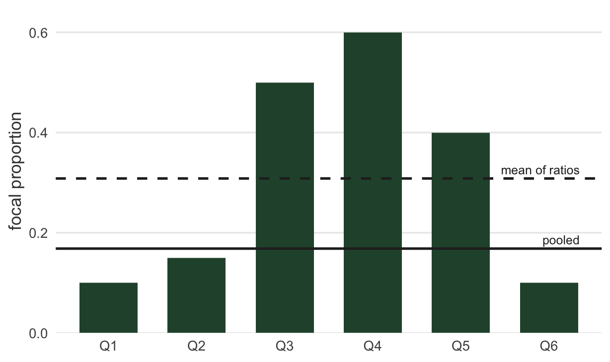
image-alt: "Bar chart of a focal species' proportion in six quadrats, with two horizontal reference lines for the pooled proportion and the mean of proportions."
---
*Updated 27 September 2026: a new section, When summarise() keeps a grouping, shows how the grouping that summarise() leaves behind turns the next summary on this survey into one row per habitat, and three ways to drop it.*
Once your field data is a tidy table, most questions become grouped summaries: mean abundance per habitat, species richness per site, the proportion of a focal species per plot. R makes this a one-liner with `dplyr`, and that is exactly why it is dangerous. The one-liner hides a choice, and the wrong choice gives you a number that answers a different question than the one you asked.
This post covers `group_by()` and `summarise()`, then spends most of its time on one measurable trap that catches ecologists constantly: the mean of per-site ratios is not the same as the ratio computed on the pooled totals, and when sampling effort differs between sites the two can differ by nearly a factor of two.
## group_by() then summarise()
The pattern is always the same. You split the rows into groups, then collapse each group to one number. Here is a focal-species survey across six quadrats in two habitats, where each quadrat has a total arthropod count (the sampling effort varies) and a count of the focal beetle:
```{r}
#| label: data
#| message: false
library(dplyr)
surv <- data.frame(
  quadrat = c("Q1", "Q2", "Q3", "Q4", "Q5", "Q6"),
  habitat = c("edge", "edge", "interior", "interior", "interior", "edge"),
  total   = c(200,  180,   40,   30,   25,  220),   # all arthropods counted
  focal   = c( 20,   27,   20,   18,   10,   22)    # the focal beetle
)
surv
```
`group_by()` marks which rows belong together and `summarise()` reduces each group to one row. `n()` counts the rows in a group; `sum()` and `mean()` do the obvious. Collapsing by habitat:
```{r}
#| label: by-habitat
surv |>
  group_by(habitat) |>
  summarise(quadrats = n(), individuals = sum(total), focal_total = sum(focal))
```
The same verbs work on an ungrouped table, which is what you want when the quadrat itself is the unit. To get the focal proportion in each quadrat, add a column with `mutate()`:
```{r}
#| label: per-quadrat
surv <- surv |> mutate(prop = focal / total)
round(surv$prop, 3)
```
The six proportions run from `r sprintf("%.2f", min(surv$prop))` to `r sprintf("%.2f", max(surv$prop))`. Now suppose you want a single headline number: what fraction of the community is the focal beetle? There are two ways to compute it, and they are not the same number.
## The mean of ratios is not the ratio of means
```{r}
#| label: two-summaries
summary_tbl <- surv |>
  summarise(
    pooled         = sum(focal) / sum(total),  # ratio of the pooled totals
    mean_of_ratios = mean(focal / total),      # average of the per-quadrat proportions
    n              = n()
  )
summary_tbl
```
```{r}
#| label: gap-numbers
#| include: false
pooled <- sum(surv$focal) / sum(surv$total)
mor <- mean(surv$focal / surv$total)
ratio <- mor / pooled
rho <- cor(surv$total, surv$prop)
wm <- weighted.mean(surv$prop, surv$total)
```
The **pooled** proportion is `r sprintf("%.3f", pooled)`: of the `r sum(surv$total)` individuals counted across all quadrats, `r sum(surv$focal)` were the focal beetle. The **mean of ratios** is `r sprintf("%.3f", mor)`, the plain average of the six per-quadrat proportions. They differ by a factor of `r sprintf("%.2f", ratio)`, and neither is a rounding artefact.
The reason is that the quadrats are not the same size and the focal proportion depends on size. The correlation between quadrat total and focal proportion is `r sprintf("%.2f", rho)`: the beetle makes up a large share of the small, sparse quadrats and a small share of the big ones. The pooled proportion is dominated by the big quadrats (they contribute most of the individuals), so it lands low. The mean of ratios gives every quadrat one equal vote regardless of size, so the small high-proportion quadrats pull it up.
Neither number is wrong. They answer different questions:
- The **pooled** proportion answers "across all the individuals I counted, what fraction is the focal species?" It is a population-level quantity, weighted by how many individuals each quadrat contributed.
- The **mean of ratios** answers "in a typical quadrat, what fraction is the focal species?" It weights quadrats equally, which is what you want if the quadrat is your unit of replication and their sizes are incidental.
The mistake is reporting one while describing the other: writing "the focal beetle is `r sprintf("%.0f", mor*100)` per cent of the community" (the mean of ratios) when "the community" means the pooled individuals (`r sprintf("%.0f", pooled*100)` per cent), or claiming "a typical quadrat is `r sprintf("%.0f", pooled*100)` per cent focal" when the per-quadrat proportions average `r sprintf("%.0f", mor*100)` per cent.
## The pooled proportion is a weighted mean
The two summaries are not unrelated. The pooled proportion is exactly the mean of the per-quadrat proportions **weighted by quadrat total**:
```{r}
#| label: weighted-mean
weighted.mean(surv$prop, w = surv$total) # equals the pooled proportion
```
This lands on `r sprintf("%.3f", wm)`, the pooled value again. So the real question behind the trap is: what should the weights be? If each individual should count equally, weight by effort (the pooled proportion). If each site should count equally, do not weight (the mean of ratios). Deciding that is ecology, not arithmetic, and `summarise()` will happily give you either without asking.
```{r}
#| label: fig-props
#| echo: false
#| fig-width: 6.4
#| fig-height: 3.8
#| fig-cap: "Focal-species proportion in each quadrat (bars), with the pooled proportion (solid line) and the mean of proportions (dashed line). The two summaries straddle the bars because the small high-proportion quadrats pull the unweighted mean up, while the pooled value follows the large quadrats."
#| fig-alt: "Bar chart of focal proportion for six quadrats ranging from 0.10 to 0.60, with a solid horizontal line near 0.17 for the pooled proportion and a dashed horizontal line near 0.31 for the mean of proportions."
library(ggplot2)
te_green <- "#275139"
ggplot(surv, aes(x = quadrat, y = prop)) +
geom_col(fill = te_green, width = 0.66) +
geom_hline(yintercept = pooled, linewidth = 0.9, colour = "grey15") +
geom_hline(yintercept = mor, linewidth = 0.9, linetype = "dashed", colour = "grey15") +
annotate("text", x = 6.35, y = pooled, label = "pooled", hjust = 1, vjust = -0.5, size = 3.3, colour = "grey15") +
annotate("text", x = 6.35, y = mor, label = "mean of ratios", hjust = 1, vjust = -0.5, size = 3.3, colour = "grey15") +
scale_y_continuous(expand = expansion(mult = c(0, 0.08))) +
labs(x = NULL, y = "focal proportion") +
theme_minimal(base_size = 13) +
theme(plot.background = element_rect(fill = "#f5f4ee", colour = NA),
panel.background = element_rect(fill = "#f5f4ee", colour = NA),
panel.grid.minor = element_blank(),
panel.grid.major.x = element_blank(),
axis.title = element_text(colour = "grey25"))
```
## When summarise() keeps a grouping
`group_by()` takes more than one column. Say you first total each quadrat within its habitat, then want one pooled proportion for the whole survey. (Each quadrat is already one row here, so the first step changes no counts. With one row per visit it would.)
```{r}
#| label: per-q
per_q <- surv |>
  group_by(habitat, quadrat) |>
  summarise(focal = sum(focal), total = sum(total))
group_vars(per_q)
```
dplyr prints a message under this chunk. It is a message, not a warning and not an error: the table is correct. It says the output is still grouped by `habitat`. `summarise()` removed only the last grouping column, `quadrat`, and `group_vars()` confirms what is left. The exact wording depends on the dplyr version (it changed in dplyr 1.2.0; this page was built with dplyr `r packageVersion("dplyr")`). The leftover grouping matters at the next step:
```{r}
#| label: leftover
by_hab <- per_q |> summarise(pooled = sum(focal) / sum(total))
by_hab
share_sum <- per_q |> mutate(share = focal / sum(focal)) |> pull(share) |> sum()
share_sum
```
The pooled proportion comes back as one row per habitat: `r sprintf("%.3f", by_hab$pooled[1])` for `r by_hab$habitat[1]` and `r sprintf("%.3f", by_hab$pooled[2])` for `r by_hab$habitat[2]`, not the survey-wide `r sprintf("%.3f", pooled)`. Average the two rows and you get `r sprintf("%.3f", mean(by_hab$pooled))`, far from the pooled value. It also lands close to the mean of ratios (`r sprintf("%.3f", mor)`), but only because both habitats have `r min(table(surv$habitat))` quadrats and the quadrats within a habitat are of similar size. On another survey the two need not agree. Each habitat gets one equal vote, although edge quadrats hold `r sum(surv$total[surv$habitat == "edge"])` of the `r sum(surv$total)` individuals. It is the trap from the section above, reached by accident. The share column fails the same way: inside the grouped `mutate()`, `sum(focal)` is a habitat total, so the shares add up to `r sprintf("%.0f", share_sum)`, one per habitat, not 1.
Three small changes remove the grouping. Each gives back the pooled proportion:
```{r}
#| label: three-fixes
surv |>
  group_by(habitat, quadrat) |>
  summarise(focal = sum(focal), total = sum(total), .groups = "drop") |>
  summarise(pooled = sum(focal) / sum(total))
per_q |> ungroup() |> summarise(pooled = sum(focal) / sum(total))
surv |>
  summarise(focal = sum(focal), total = sum(total), .by = c(habitat, quadrat)) |>
  summarise(pooled = sum(focal) / sum(total))
```
`.groups = "drop"` removes every grouping when `summarise()` finishes. `ungroup()` removes it afterwards. `.by` groups for this one call only (it needs dplyr 1.1.0 or newer), and the table it returns is not grouped, so nothing is left over. (The third result prints as a plain data frame because `surv` is one; the number is the same.) `.by` refuses a table that is already grouped. That is an error, which stops a script; here `tryCatch()` catches it so the page can print its text:
```{r}
#| label: by-on-grouped
tryCatch(per_q |> summarise(pooled = sum(focal) / sum(total), .by = habitat),
         error = function(e) conditionMessage(e))
```
```{r}
#| label: grouping-checks
#| include: false
msgs <- character(0); warns <- 0
again <- withCallingHandlers(
surv |> group_by(habitat, quadrat) |> summarise(focal = sum(focal), total = sum(total)),
message = function(m) { msgs <<- c(msgs, conditionMessage(m)); invokeRestart("muffleMessage") },
warning = function(w) { warns <<- warns + 1; invokeRestart("muffleWarning") })
stopifnot(length(msgs) == 1, grepl("habitat", msgs), warns == 0, identical(group_vars(per_q), "habitat"))
stopifnot(nrow(per_q) == nrow(surv), nrow(by_hab) == 2, isTRUE(all.equal(share_sum, n_distinct(surv$habitat))))
fix_drop <- surv |> group_by(habitat, quadrat) |> summarise(focal = sum(focal), total = sum(total), .groups = "drop")
fix_by <- surv |> summarise(focal = sum(focal), total = sum(total), .by = c(habitat, quadrat))
stopifnot(!is_grouped_df(fix_drop), !is_grouped_df(fix_by), is.data.frame(fix_by), !inherits(fix_by, "tbl_df"))
for (tab in list(fix_drop, ungroup(per_q), fix_by)) stopifnot(all.equal(sum(tab$focal) / sum(tab$total), pooled))
stopifnot(inherits(tryCatch(summarise(per_q, n = n(), .by = habitat), error = function(e) e), "error"))
stopifnot(length(unique(table(surv$habitat))) == 1, all(tapply(surv$total, surv$habitat, function(x) max(x) / min(x)) < 2))
stopifnot(packageVersion("dplyr") >= "1.1.0")
```
## Where to go next
Grouped summaries assume the table is already assembled, but survey data usually arrives in two tables, one for sites and one for observations, that you have to join. The next trap lives there: an inner join silently drops the sites where the species was absent, which biases exactly the kind of mean you just computed. The joining tutorial takes that apart.
## References
Wickham H, Averick M, Bryan J, et al 2019. Journal of Open Source Software 4(43):1686 (10.21105/joss.01686).
Wickham H, Cetinkaya-Rundel M, Grolemund G 2023. R for Data Science, 2nd ed. O'Reilly. ISBN 978-1-492-09740-2.
## Related tutorials
- [Per chick or per nest: informative cluster size](../informative-cluster-size/)
- [Repeating an analysis for every site in R](../repeating-an-analysis-for-every-site/)
- [Joining ecological tables without losing zeros](../joining-ecological-tables/)
- [From a field sheet to your first analysis](../from-field-sheet-to-first-analysis/)