library(ggplot2); library(dplyr); library(tidyr)
te <- c(forest = "#2f5d50", moss = "#7a9b76", rust = "#b5651d", gold = "#c9a227",
        slate = "#3d4b53", sand = "#d9cbb2", sky = "#5b8aa6", brick = "#8c3b2e")
theme_te <- function(base_size = 12) {
  theme_minimal(base_size = base_size) +
    theme(panel.grid.minor = element_blank(),
          panel.grid.major = element_line(colour = "#e7e1d5", linewidth = 0.3),
          axis.title = element_text(colour = "#3d4b53"),
          axis.text  = element_text(colour = "#5c6670"),
          plot.title = element_text(colour = "#2f3a40", face = "bold", size = base_size + 1),
          plot.subtitle = element_text(colour = "#5c6670", size = base_size - 1),
          legend.position = "bottom",
          legend.title = element_text(colour = "#3d4b53"),
          plot.background  = element_rect(fill = "#f5f4ee", colour = NA),
          panel.background = element_rect(fill = "#f5f4ee", colour = NA))
}Coverage-based rarefaction and extrapolation
R
species richness
biodiversity
ecology tutorial
Comparing richness at equal sample size can rank two assemblages the wrong way. Standardise by coverage instead, in base R, and see where extrapolation stops.
Updated 25 September 2026: a new section, Good’s coverage, and what 0.98 does not mean, shows on a community of known make-up that coverage is the share of individuals belonging to species already seen, not the share of species found, and how far Good’s estimate runs low on average.
Two samples, different numbers of individuals, and you want to know which assemblage is richer. The reflex is to rarefy both down to the same number of individuals and compare. That is the right instinct about sample size, but it can still give the wrong answer, because two samples of the same size can differ in how completely they cover their communities. The fix, from Chao and Jost, is to standardise by sample coverage rather than by count. This post builds rarefaction, extrapolation and coverage from scratch and compares the same two samples on both bases.
The building blocks
Three functions carry the whole post. Rarefied richness is Hurlbert’s expectation: the mean number of species in a random subsample of m individuals. Rarefied coverage is the expected sample coverage of that subsample. Sample coverage itself, the fraction of the community’s individuals that belong to species you sampled, comes from a Good-Turing formula, improved by Chao and Jost with the doubletons term.
lchoose_safe <- function(n, k) ifelse(k > n | k < 0, -Inf, lchoose(n, k))
rare_S <- function(x, m)                                   # Hurlbert rarefied richness
  sapply(m, function(mm) { n <- sum(x)
    sum(1 - exp(lchoose_safe(n - x, mm) - lchoose_safe(n, mm))) })
rare_C <- function(x, m) {                                 # rarefied sample coverage
  n <- sum(x)
  sapply(m, function(mm)                                   # the formula holds for m < n only;
    if (mm >= n) covhat(x) else                            # at m = n it is the Good-Turing value
      1 - sum((x / n) * exp(lchoose_safe(n - x, mm) - lchoose_safe(n - 1, mm))))
}
covhat <- function(x) { n <- sum(x); f1 <- sum(x == 1); f2 <- sum(x == 2)
  if (f2 == 0) f2 <- f1 * (f1 - 1) / 2
  1 - (f1 / n) * ((n - 1) * f1 / ((n - 1) * f1 + 2 * f2)) }
chao1  <- function(x) { n <- sum(x); f1 <- sum(x == 1); f2 <- sum(x == 2)
  length(x) + (n - 1) / n * f1 * (f1 - 1) / (2 * (f2 + 1)) }
extr_S <- function(x, m) { n <- sum(x); f1 <- sum(x == 1); f2 <- sum(x == 2)
  f0 <- (n - 1) / n * f1 * (f1 - 1) / (2 * (f2 + 1)); So <- length(x)
  sapply(m, function(mm) if (mm <= n)
    sum(1 - exp(lchoose_safe(n - x, mm) - lchoose_safe(n, mm)))
    else So + f0 * (1 - (1 - f1 / (n * f0 + f1))^(mm - n))) }
Good’s coverage, and what 0.98 does not mean
Good’s coverage is 1 - f1/n, where f1 is the number of species seen exactly once and n is the number of individuals in the sample (Good 1953). It estimates the share of the community’s individuals that belong to species already in the sample. It does not estimate the share of species you have found. A coverage of 0.98 says that the next individual you catch has about a 2 per cent chance of belonging to a species not yet in the sample; it says little about how many species are still missing, because the missing ones are rare.
To see the gap, draw samples of increasing size from a known community: the lognormal assemblage of 180 species used in Checking a diversity estimate. For every sample, record Good’s estimate, the Chao and Jost version used in this post (covhat()), the true coverage (the summed relative abundance of the species the sample caught) and the share of the 180 species it caught.
set.seed(4193)                                       # same community as the checking post
S_known   <- 180
rel_known <- exp(rnorm(S_known, 0, 1.6)); rel_known <- rel_known / sum(rel_known)
good_cov  <- function(x) 1 - sum(x == 1) / sum(x)   # Good's (Turing's) estimator

sizes_cov <- c(50, 100, 250, 500, 1500, 5000); reps_cov <- 2000
cov_draws <- lapply(sizes_cov, function(nn) t(replicate(reps_cov, {
  x_s  <- as.vector(rmultinom(1, nn, rel_known)); seen <- x_s > 0
  c(good = good_cov(x_s[seen]), chao_jost = covhat(x_s[seen]),
    true_coverage = sum(rel_known[seen]), species_seen = mean(seen)) })))
cov_table <- data.frame(n = sizes_cov, t(sapply(cov_draws, colMeans)))
cov_err   <- sapply(cov_draws, function(d) d[, "good"] - d[, "true_coverage"])
cov_bias  <- colMeans(cov_err)                       # mean error of Good's estimate
cov_bias_se <- apply(cov_err, 2, sd) / sqrt(reps_cov)
cov_mae   <- colMeans(abs(cov_err))                  # typical error of one sample
cj_shift  <- abs(cov_table$chao_jost - cov_table$good)
rare_2pc  <- sum(cumsum(sort(rel_known)) <= 0.02)    # rarest species holding 2 per cent
good_shortfall <- sapply(sizes_cov, function(nn)    # exact E(true coverage) - E(Good)
  sum(rel_known^2 * (1 - rel_known)^(nn - 1)))
cov_z     <- (cov_bias + good_shortfall) / cov_bias_se  # simulation against the formula
round(cov_table, 3)
n good chao_jost true_coverage species_seen
1 50 0.578 0.583 0.579 0.174
2 100 0.729 0.731 0.729 0.268
3 250 0.866 0.866 0.866 0.423
4 500 0.927 0.927 0.928 0.558
5 1500 0.979 0.979 0.979 0.772
6 5000 0.997 0.997 0.997 0.929data.frame(n = sizes_cov, exact_gap = round(good_shortfall, 4),
simulated_gap = round(-cov_bias, 4), mc_se = round(cov_bias_se, 4)) n exact_gap simulated_gap mc_se
1 50 0.0048 0.0016 0.0022
2 100 0.0019 0.0006 0.0015
3 250 0.0004 0.0004 0.0007
4 500 0.0001 0.0006 0.0004
5 1500 0.0000 0.0000 0.0001
6 5000 0.0000 0.0000 0.0000Good’s estimate needs no simulation to judge on average. With p the relative abundance of a species, the expected number of singletons is the sum of n p (1 - p)^(n - 1) over the species and the expected uncovered share is the sum of p (1 - p)^n, so 1 - f1/n runs low on average by the sum of p^2 (1 - p)^(n - 1). For this community that is 0.0048 at n = 50 and 0.0004 at n = 250 (the exact_gap column). Every simulated average, over 2000 samples per size, lies within 1.5 Monte Carlo standard errors of that value, but at n = 50 the standard error, 0.0022, is about half the exact gap, so the simulation alone could not pin its size down. A single sample scatters far more: its absolute error averages 0.078 at n = 50 and 0.013 at n = 500. The Chao and Jost term raises the estimate by 0.0050 on average at n = 50, about the size of that shortfall, and by at most 0.0004 from n = 250 up.
The last two columns of the first table part company. At n = 1500 a sample covers on average 0.979 of the individuals but holds only 77 per cent of the species; at n = 5000 the figures are 0.997 and 93 per cent. The reason is in the community: its rarest 53 species together hold less than 2 per cent of the individuals, so a sample can miss every one of them and still cover 98 per cent of the individuals. The expected number of species that a sample of 1500 misses is the sum of (1 - p)^1500 over the species: 41 of the 180.
Chao and colleagues (2020) put the two quantities into one sample completeness profile: at order q = 0 completeness is the share of species detected, at q = 1 it is coverage. Standardising by coverage, as the rest of this post does, makes samples equally complete in the second sense, not the first. If the question is how many species are missing, you need an estimate of the undetected ones, which is extrapolation (Estimating species richness beyond your sample).
Two assemblages, same effort
Assemblage A is species-poor but even; assemblage B is richer but dominated by a few common species with a long tail of rarities. Both are sampled with 250 individuals.
set.seed(13)
SA <- 90;  relA <- exp(rnorm(SA, 0, 0.55)); relA <- relA / sum(relA)
SB <- 200; relB <- exp(rnorm(SB, 0, 1.70)); relB <- relB / sum(relB)
n <- 250
xA <- as.vector(rmultinom(1, n, relA)); xA <- xA[xA > 0]
xB <- as.vector(rmultinom(1, n, relB)); xB <- xB[xB > 0]
SobsA <- length(xA); SobsB <- length(xB); CA <- covhat(xA); CB <- covhat(xB)
round(c(SobsA = SobsA, SobsB = SobsB, coverageA = CA, coverageB = CB), 4)
SobsA SobsB coverageA coverageB
74.0000 68.0000 0.9325 0.8524 At equal size you have two raw counts. Assemblage A shows 74 species, assemblage B shows 68. Neither reaches the truth: A has 90 species and B has 200. The clue is coverage. A is sampled to 0.933 coverage and B to 0.852: B’s curve is still climbing steeply, its rare tail barely touched, so its 68 is a far worse snapshot of the truth than A’s 74.
Extrapolation past the reference sample
Rarefaction runs the sample down; extrapolation runs it up, using the Chao1 estimate of unseen species to project where the curve is heading. Reliable extrapolation reaches only about twice the reference sample size, so we stop at 500.
SA_2 <- extr_S(xA, 2 * n); SB_2 <- extr_S(xB, 2 * n)
c(A_at_500 = round(SA_2, 1), B_at_500 = round(SB_2, 1),
  Chao1_A = round(chao1(xA), 1), Chao1_B = round(chao1(xB), 1))
A_at_500 B_at_500 Chao1_A Chao1_B
80.7 94.3 81.5 119.0 Projected to 500 individuals, A reaches 80.7 and B reaches 94.3. A comparison made at 250 individuals is a comparison at one point on two curves that are still moving. The Chao1 asymptotes are 81.5 for A and 119 for B.
grid <- seq(1, 2 * n, by = 5)
mk <- function(x, lab) data.frame(m = grid, S = extr_S(x, grid), assemblage = lab,
                                  part = ifelse(grid <= n, "interpolation", "extrapolation"))
allc <- rbind(mk(xA, "A (even, true S = 90)"), mk(xB, "B (uneven, true S = 200)"))
cols <- c("A (even, true S = 90)" = unname(te["forest"]),
          "B (uneven, true S = 200)" = unname(te["rust"]))
p_curves <- ggplot(allc, aes(m, S, colour = assemblage)) +
  geom_vline(xintercept = n, linetype = "dotted", colour = te["slate"], linewidth = 0.4) +
  geom_line(aes(linetype = part), linewidth = 0.9) +
  geom_point(data = data.frame(m = n, S = c(SobsA, SobsB),
             assemblage = names(cols)), size = 3, show.legend = FALSE) +
  annotate("text", x = n, y = 20, label = "reference sample n = 250",
           angle = 90, vjust = -0.4, hjust = 0, size = 3, colour = te["slate"]) +
  scale_colour_manual(values = cols, name = NULL) +
  scale_linetype_manual(values = c("interpolation" = "solid", "extrapolation" = "22"), name = NULL) +
  labs(title = "Size-based rarefaction and extrapolation for two assemblages",
       subtitle = "Solid = interpolation, dashed = extrapolation",
       x = "number of individuals", y = "expected species richness") +
  theme_te()
p_curves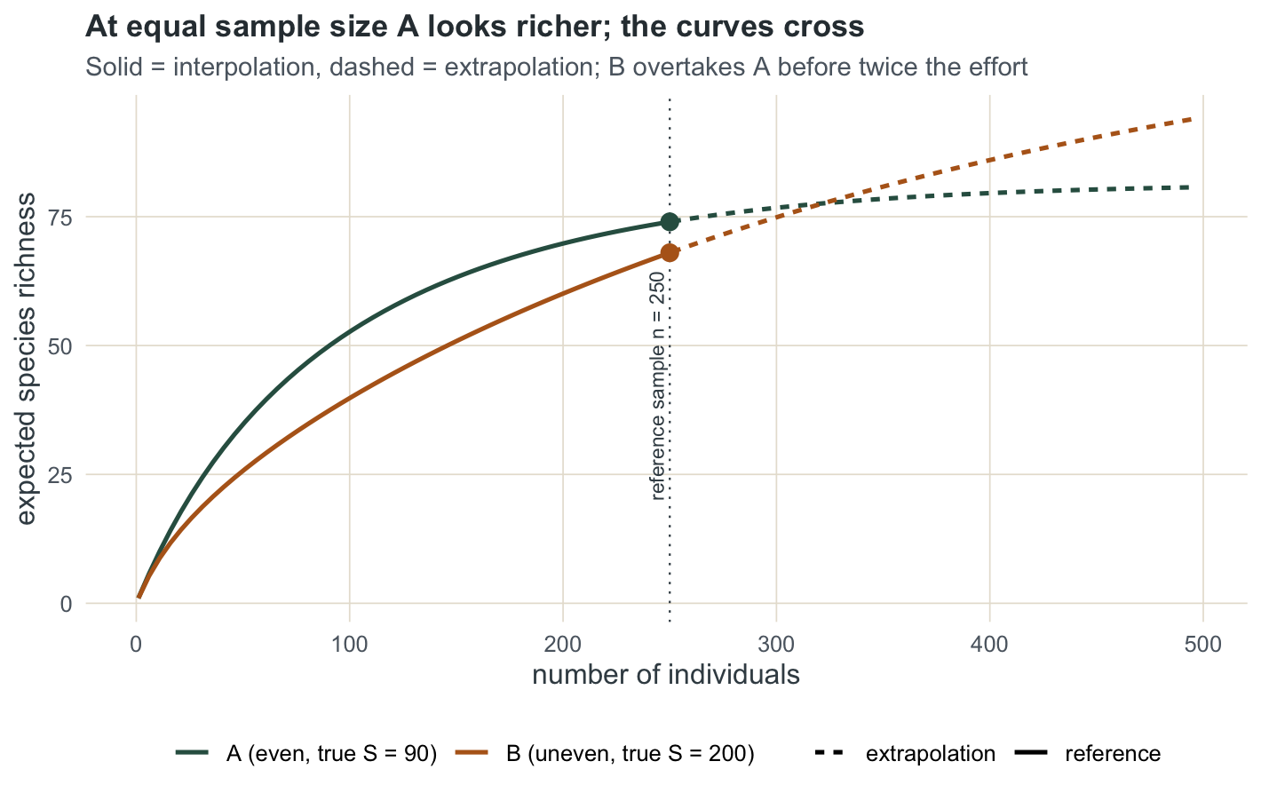
Standardising by coverage instead of size
The principled comparison holds coverage constant, not size. Bring both samples to the coverage of the less complete one, 0.8524, by rarefying A down until it reaches that coverage.
Clow <- min(CA, CB)
m_for_C <- function(x, Ct) { ms <- 1:sum(x); ms[which.min(abs(rare_C(x, ms) - Ct))] }
mA_low <- m_for_C(xA, Clow)
SA_low <- rare_S(xA, mA_low)              # A rarefied to B's coverage
SB_low <- SobsB                           # B is already at this coverage
c(target_coverage = round(Clow, 4), A_richness = round(SA_low, 1),
  A_at_m = mA_low, B_richness = round(SB_low, 1))
target_coverage A_richness A_at_m B_richness
0.8524 65.0000 161.0000 68.0000 Rarefying A to coverage 0.8524 takes it down to 161 individuals and 65 species, against B’s 68. Both figures now describe samples that are equally complete in coverage rather than equally large. The equal-size comparison penalised nothing about B being under-sampled; the equal-coverage comparison removes that confound.
ms <- 1:n
cc <- rbind(
  data.frame(C = rare_C(xA, ms), S = rare_S(xA, ms), assemblage = "A (even, true S = 90)"),
  data.frame(C = rare_C(xB, ms), S = rare_S(xB, ms), assemblage = "B (uneven, true S = 200)"))
ggplot(cc, aes(C, S, colour = assemblage)) +
  geom_vline(xintercept = Clow, linetype = "dotted", colour = te["slate"], linewidth = 0.4) +
  geom_line(linewidth = 0.9) +
  geom_point(data = data.frame(C = c(CA, CB), S = c(SobsA, SobsB),
             assemblage = names(cols)), size = 3, show.legend = FALSE) +
  annotate("text", x = Clow, y = 15, label = "equal coverage 0.852",
           angle = 90, vjust = 1.2, hjust = 0, size = 3, colour = te["slate"]) +
  scale_colour_manual(values = cols, name = NULL) +
  # zoom the axis, do not subset the data: scale limits would censor the points outside
  # the window and stop each line short of the panel edge
  coord_cartesian(xlim = c(0.3, 0.95)) +
  labs(title = "Expected richness against sample coverage",
       subtitle = "Dotted line = the lower of the two sample coverages",
       x = "sample coverage", y = "expected species richness") +
  theme_te()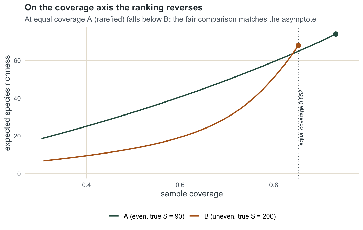
Where it stops
Coverage-based standardisation makes the comparison fair, but it does not conjure the truth. It compares richness up to the shared coverage; it does not recover B’s full 200 species, because those rarest species are simply not in the sample. Extrapolation can reach a little past the data, to roughly twice the sample size, and no further with any confidence: push it and you are reading the estimator’s assumptions, not the community. Comparing samples fairly and estimating true richness are two different jobs, and the second is always bounded by what you sampled. The next tutorial takes the same limit into the wider diversity profile.
References
Hurlbert S H 1971 Ecology 52(4):577-586 (10.2307/1934145)
Good I J 1953 Biometrika 40(3-4):237-264 (10.1093/biomet/40.3-4.237)
Chao A, Jost L 2012 Ecology 93(12):2533-2547 (10.1890/11-1952.1)
Colwell R K, Chao A, Gotelli N J, Lin S-Y, Mao C X, Chazdon R L, Longino J T 2012 Journal of Plant Ecology 5(1):3-21 (10.1093/jpe/rtr044)
Chao A, Gotelli N J, Hsieh T C, Sander E L, Ma K H, Colwell R K, Ellison A M 2014 Ecological Monographs 84(1):45-67 (10.1890/13-0133.1)
Hsieh T C, Ma K H, Chao A 2016 Methods in Ecology and Evolution 7(12):1451-1456 (10.1111/2041-210X.12613)
Chao A, Kubota Y, Zeleny D, Chiu C-H, Li C-F, Kusumoto B, Yasuhara M, Thorn S, Wei C-L, Costello M J, Colwell R K 2020 Ecological Research 35(2):292-314 (10.1111/1440-1703.12102)