---
title: "Fitting species abundance distributions in R"
description: "Fit and compare rank-abundance (dominance/diversity) models in R with vegan's radfit: niche pre-emption, lognormal, Zipf and Zipf-Mandelbrot, with AIC model selection and Preston octave plots for community ecology."
date: "2026-06-24 13:00"
categories: [R, community ecology, biodiversity, vegan]
image: thumbnail.png
image-alt: "Rank-abundance curves for two ecological communities with fitted SAD models on a log abundance axis"
---
A diversity index turns a whole community into one number. Shannon, Simpson and evenness are useful, but they throw away the shape of the abundance distribution: how steeply the common species tower over the rare ones, and whether there is a mode in the middle. That shape is the species abundance distribution (SAD), one of the oldest descriptions in community ecology (Fisher et al. 1943; Preston 1948).
This post fits parametric SAD models to ranked counts with `vegan::radfit`, compares them with AIC, and shows how two communities with similar species lists end up under different models. The point is not that a fitted model reveals a mechanism. It is that the rank-abundance curve carries structure that a single index hides, and that model selection gives a compact, comparable summary of that structure.
## Two synthetic communities
The data are illustrative. One community has strong dominance, like an early-successional site where one or two species pre-empt most of the available space. The other is more even, with many species of intermediate abundance and a few rare ones, closer to a mature stand.
```{r}
#| label: data
#| message: false
#| warning: false
library(vegan)
library(ggplot2)
library(dplyr)
library(tidyr)

# Quarry: early-successional, niche pre-emption (geometric dominance).
# Each species takes a fixed fraction k of the resource left by the previous one.
set.seed(19)
S1 <- 15; k <- 0.38; Ntot1 <- 2600
rem <- 1; props <- numeric(S1)
for (i in 1:S1) { props[i] <- k * rem; rem <- rem - props[i] }
props <- props / sum(props)
quarry <- rpois(S1, props * Ntot1); quarry <- quarry[quarry > 0]

# Forest: mature, lognormal SAD (more even, with an internal mode in log abundance).
set.seed(204)
raw <- rlnorm(55, meanlog = 1.7, sdlog = 1.05)
forest <- round(raw * 4200 / sum(raw)); forest <- forest[forest > 0]

c(quarry_S = length(quarry), quarry_N = sum(quarry),
  forest_S = length(forest), forest_N = sum(forest))
```
The quarry holds `r length(quarry)` species in `r sum(quarry)` individuals; the forest holds `r length(forest)` species in `r sum(forest)`. Sorted from most to least abundant, the quarry falls away fast (951 down to a single individual), while the forest descends more gently.
## What the indices say, and what they hide
```{r}
#| label: indices
idx <- function(x) {
  H <- diversity(x, "shannon")
  data.frame(
    S = sum(x > 0), N = sum(x),
    Shannon = round(H, 2),
    Simpson = round(diversity(x, "simpson"), 3),
    Pielou_J = round(H / log(sum(x > 0)), 2),
    Hill_q1 = round(exp(H), 1))
}
knitr::kable(rbind(Quarry = idx(quarry), Forest = idx(forest)))
```
The forest is more diverse and far more even (Pielou's J of 0.88 against 0.66). These numbers tell you the forest is flatter, but they do not tell you the form of the flattening: whether the abundances decline geometrically, follow a lognormal hump, or fall on a power law. For that you need the curve itself.
## Rank-abundance curves and the radfit models
A rank-abundance (dominance/diversity) plot puts species rank on the x-axis and abundance on a log y-axis (Whittaker 1965). `radfit` fits five models to these ranked counts as Poisson generalized linear models, choosing parameters by minimizing deviance (Wilson 1991):
- **Null** (broken stick): no free parameters, a neutral partition of the resource axis.
- **Pre-emption** (geometric series): one parameter, a constant fraction taken at each rank. A straight line on the log axis.
- **Lognormal**: two parameters, a hump in log abundance.
- **Zipf**: two parameters, a power law with a heavy tail of rare species.
- **Zipf-Mandelbrot**: three parameters, a more flexible version of Zipf.
```{r}
#| label: radfit
#| message: false
#| warning: false
rq <- radfit(quarry)
rf <- radfit(forest)
rq
rf
```
```{r}
#| label: fig-rad
#| fig-width: 8.6
#| fig-height: 4.2
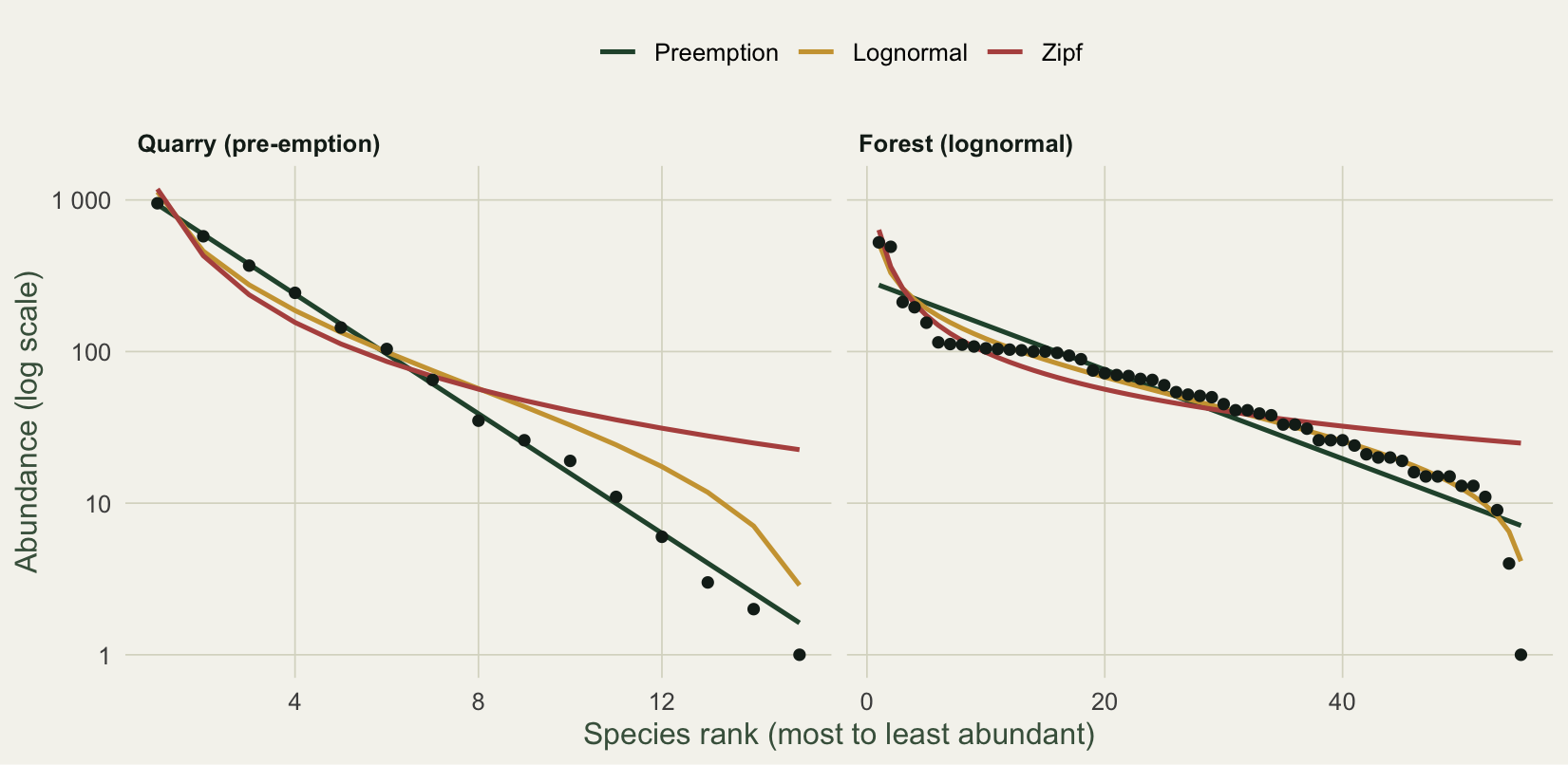
#| fig-cap: "Rank-abundance curves with three fitted SAD models. The quarry follows a straight pre-emption line on the log axis; the forest bends away from it toward a lognormal."
#| fig-alt: "Rank-abundance curves for two communities on a log axis with fitted SAD models: the quarry follows a straight pre-emption line while the forest bends toward a lognormal."
ink <- "#16241d"; forest_col <- "#275139"; gold <- "#cda23f"; red <- "#b5534e"
faint <- "#5d6b61"; line_col <- "#dad9ca"; paper <- "#f5f4ee"

fitcurve <- function(r, model, site) {
  f <- r$models[[model]]$fitted.values
  data.frame(rank = seq_along(f), fit = f, model = model, site = site)
}
mods <- c("Preemption", "Lognormal", "Zipf")
fit <- bind_rows(
  lapply(mods, fitcurve, r = rq, site = "Quarry (pre-emption)"),
  lapply(mods, fitcurve, r = rf, site = "Forest (lognormal)"))
obs <- bind_rows(
  data.frame(rank = seq_along(quarry), abund = sort(quarry, decreasing = TRUE),
             site = "Quarry (pre-emption)"),
  data.frame(rank = seq_along(forest), abund = sort(forest, decreasing = TRUE),
             site = "Forest (lognormal)"))
lev <- c("Quarry (pre-emption)", "Forest (lognormal)")
fit$site <- factor(fit$site, lev); obs$site <- factor(obs$site, lev)
fit$model <- factor(fit$model, levels = mods)

te <- theme_minimal(base_size = 12) + theme(
  panel.grid.minor = element_blank(),
  panel.grid.major = element_line(color = line_col, linewidth = 0.3),
  plot.background = element_rect(fill = paper, color = NA),
  panel.background = element_rect(fill = paper, color = NA),
  strip.text = element_text(face = "bold", color = ink, hjust = 0),
  axis.title = element_text(color = "#46604a"),
  legend.position = "top", legend.title = element_blank())

ggplot() +
  geom_line(data = fit, aes(rank, fit, color = model), linewidth = 0.9) +
  geom_point(data = obs, aes(rank, abund), color = ink, size = 1.6) +
  facet_wrap(~site, scales = "free_x") +
  scale_y_log10(labels = scales::label_number()) +
  scale_color_manual(values = c(Preemption = forest_col, Lognormal = gold, Zipf = red)) +
  labs(x = "Species rank (most to least abundant)", y = "Abundance (log scale)") + te
```
For the quarry, pre-emption wins outright: an AIC of 88.3 against 250.5 for the lognormal and 980.1 for the null. The fitted fraction is about 0.36, so each species in rank order holds roughly a third of what the one above it held. On the log axis that is a straight line, and the points sit on it. For the forest the order reverses: the lognormal wins (AIC 475.5), the pre-emption model is the worst fit (879.3), and the points trace the gentle S-curve that a geometric series cannot follow.
## The Preston octave plot
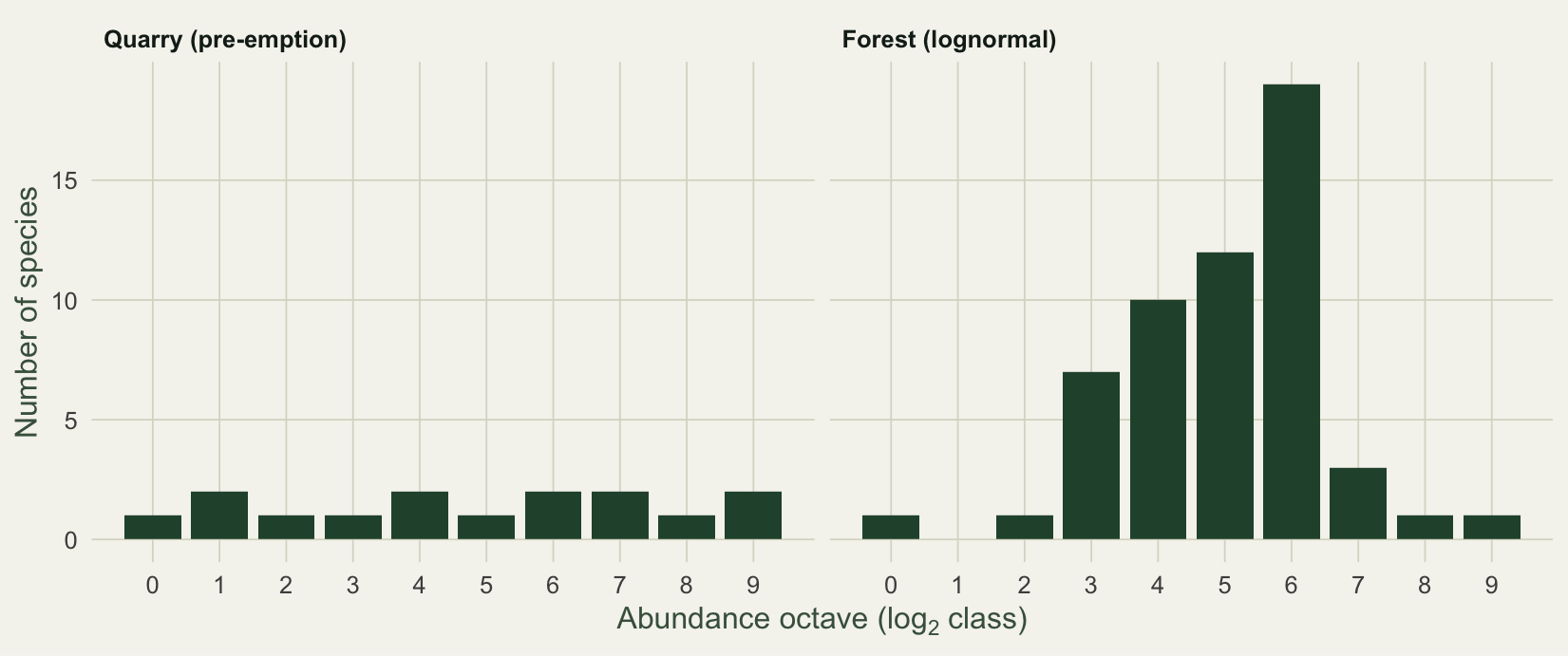
Preston (1948) binned species into octaves, doubling abundance classes (1, 2 to 3, 4 to 7, and so on). A lognormal community shows an internal mode: a peak at some intermediate octave, with fewer species both rarer and commoner. A geometric community has no such peak; species are spread roughly evenly across octaves.
```{r}
#| label: fig-octave
#| fig-width: 8.6
#| fig-height: 3.6
#| fig-cap: "Preston octave plots. The forest has a clear internal mode near octave 6, the signature of a lognormal; the quarry is flat across octaves."
#| fig-alt: "Preston octave plots of species counts: the forest shows an internal peak near octave six while the quarry stays flat across octaves."
octdf <- function(x, site) {
  cl <- floor(log2(sort(x, decreasing = TRUE)))
  tb <- tabulate(cl + 1, nbins = max(cl) + 1)
  data.frame(octave = seq_along(tb) - 1, nsp = tb, site = site)
}
oct <- bind_rows(octdf(quarry, "Quarry (pre-emption)"),
                 octdf(forest, "Forest (lognormal)"))
oct$site <- factor(oct$site, lev)

ggplot(oct, aes(octave, nsp)) +
  geom_col(fill = forest_col, width = 0.85) +
  facet_wrap(~site) +
  scale_x_continuous(breaks = 0:9) +
  labs(x = expression(paste("Abundance octave (", log[2], " class)")),
       y = "Number of species") + te
```
The forest piles up near octave 6, exactly where a lognormal puts its mode. The quarry has no peak, which is why the lognormal fits it poorly and the geometric line fits it well.
## Model selection across all five models
Ranking by AIC makes the contrast explicit. The best model has a delta of zero; everything else is measured against it.
```{r}
#| label: fig-aic
#| fig-width: 8.6
#| fig-height: 3.4
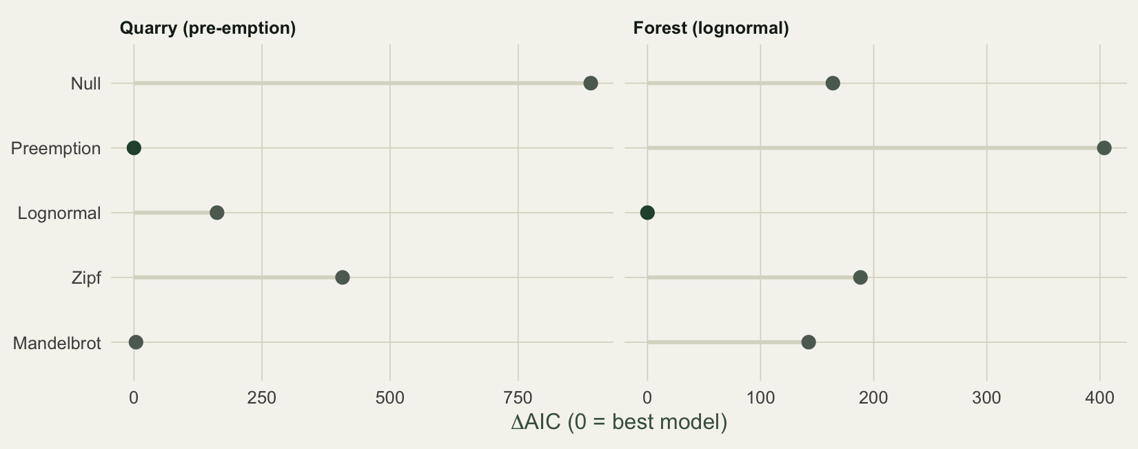
#| fig-cap: "Delta-AIC by model. Pre-emption is best for the quarry, lognormal for the forest. Zipf-Mandelbrot is close behind the winner each time but never wins, because AIC charges for its extra parameter."
#| fig-alt: "Bar chart of delta-AIC by model, with pre-emption lowest for the quarry and lognormal lowest for the forest, and Zipf-Mandelbrot always close behind but never best."
getaic <- function(r) sapply(r$models, function(m) tryCatch(AIC(m), error = function(e) NA))
aicdf <- bind_rows(
  data.frame(model = names(getaic(rq)), aic = getaic(rq), site = "Quarry (pre-emption)"),
  data.frame(model = names(getaic(rf)), aic = getaic(rf), site = "Forest (lognormal)")) %>%
  group_by(site) %>% mutate(dAIC = aic - min(aic, na.rm = TRUE), best = dAIC == 0) %>% ungroup()
aicdf$site <- factor(aicdf$site, lev)
aicdf$model <- factor(aicdf$model,
  levels = rev(c("Null", "Preemption", "Lognormal", "Zipf", "Mandelbrot")))

ggplot(aicdf, aes(dAIC, model)) +
  geom_segment(aes(x = 0, xend = dAIC, yend = model), color = line_col, linewidth = 1) +
  geom_point(aes(color = best), size = 3) +
  facet_wrap(~site, scales = "free_x") +
  scale_color_manual(values = c(`FALSE` = faint, `TRUE` = forest_col), guide = "none") +
  labs(x = expression(paste(Delta, "AIC (0 = best model)")), y = NULL) + te
```
One detail rewards attention. For the quarry, Zipf-Mandelbrot fits the data exactly as well as pre-emption: both reach a deviance of about 4.2. But Mandelbrot carries one extra parameter, so its AIC is 92.3 against 88.3, a delta of 4. Equal fit, worse score. This is parsimony in action: when two models describe the data equally well, the simpler one is preferred, and AIC does the bookkeeping. The extra flexibility of Mandelbrot only pays off in the forest, where the lognormal still beats it.
## How far to read these fits
A fitted SAD model is a description, not a diagnosis. Many processes can generate the same curve, and the SAD on its own rarely discriminates among them (McGill et al. 2007). A geometric fit is consistent with sequential niche pre-emption, but it does not prove it; a lognormal can arise from the central limit theorem acting on multiplicative growth, with no special ecology required. Treat the winning model as a compact summary of community structure that lets you compare sites, not as evidence for a mechanism.
A few practical notes. The models are fitted to ranked counts, so they describe relative abundance, not absolute density; rescale before comparing communities sampled at different efforts. With strongly geometric data the three-parameter Mandelbrot model can fail to converge and `radfit` returns `NA` for it, which is informative rather than alarming: the data do not support the extra parameters. And `radfit` works on a single community vector here, but it also accepts a site-by-species matrix and fits every row at once, which is the usual way to compare many plots.
## References
Fisher RA, Corbet AS, Williams CB (1943). The relation between the number of species and the number of individuals in a random sample of an animal population. *Journal of Animal Ecology* 12(1):42-58. doi:10.2307/1411
Preston FW (1948). The commonness and rarity of species. *Ecology* 29(3):254-283. doi:10.2307/1930989
Whittaker RH (1965). Dominance and diversity in land plant communities. *Science* 147(3655):250-260. doi:10.1126/science.147.3655.250
Wilson JB (1991). Methods for fitting dominance/diversity curves. *Journal of Vegetation Science* 2(1):35-46. doi:10.2307/3235896
McGill BJ, Etienne RS, Gray JS, et al. (2007). Species abundance distributions: moving beyond single prediction theories to integration within an ecological framework. *Ecology Letters* 10(10):995-1015. doi:10.1111/j.1461-0248.2007.01094.x
Oksanen J, Simpson G, Blanchet F, et al. (2022). *vegan: Community Ecology Package*. R package version 2.6-4.