library(ggplot2)
set.seed(298)The exact Ewens test: is your SAD neutral?
R
neutral theory
species abundance
hypothesis testing
ecology tutorial
Watterson’s exact test in R. Condition on richness, and the neutral null loses its free parameter. Measured power against three classic niche models of the SAD.
Corrected 14 October 2026: the figure caption and alt texts put the Sugihara marker in the right tail; it sits on the right shoulder, inside the range the test accepts, and they now say so. The limits section said a dispersal-limited neutral plot will fail the test and now says it can fail but can also pass; the take-away of the sample size section is now limited to niche models like this Sugihara community rather than any lognormal-shaped one; and the introduction now says that fitting a neutral curve is not by itself a test, rather than that the plot is not evidence of anything.
Corrected 1 October 2026: the sample size comparison also enlarged the Sugihara species pool, so the gain in power it reported was not the effect of more individuals alone; it now holds the pool fixed and reports the smaller gain. The identity check said every gap sat at the last bit of the double; it now says the last few bits.
Corrected 30 September 2026: the limits section said Etienne extended this exact test to multiple samples and that McGill and colleagues held that abundance distributions cannot arbitrate between theories at all; it now describes Etienne’s multi-sample test as a different test that depends on parameter values, and says McGill and colleagues noted that few abundance distribution models are ever rejected.
Corrected 27 September 2026: the closing section said two of the three niche models survive the test most of the time at J = 500; by the power table only Sugihara does, while the preemption model survives about half the time.
Fitting Hubbell’s \(\theta\) to an abundance vector uses the richness and the sample size and discards the rest. The first post in this cluster measured that: two samples with wildly different shapes and the same \(S\) and \(J\) get bit-identical fits. Which means that fitting a neutral curve to a rank abundance plot is not, by itself, a test of anything. The curve was never asked about the shape.
The same fact that causes the problem also solves it. If \(\theta\) only ever sees \(S\) and \(J\), then conditioning on \(S\) and \(J\) removes \(\theta\) from the model entirely, and what is left is a null hypothesis with no free parameters. That is Watterson’s exact test, standard in population genetics since 1978 and underused in ecology.
Setup
Conditioning kills the parameter
The Ewens formula factorises into a combinatorial constant and \(\theta^S / (\theta)_J\). Sum it over every abundance vector with exactly \(S\) species and you get
\[P(S \mid \theta, J) = \frac{|s(J,S)|}{(\theta)_J}\,\theta^S\]
where \(|s(J,S)|\) is an unsigned Stirling number of the first kind. Divide the joint by the marginal and the \(\theta\) cancels:
\[P(n_1,\dots,n_S \mid S, J) = \frac{J!}{\prod_i n_i \prod_j \Phi_j! \; |s(J,S)|}\]
No \(\theta\) anywhere on the right. The cancellation rests on an identity, and identities are cheap to check, so check it: sum the combinatorial term over every partition of \(J\) into exactly \(S\) parts and you should land on \(|s(J,S)|\).
log_stirling1 <- function(N) {
  L <- matrix(-Inf, N + 1, N + 1); L[1, 1] <- 0
  for (n in 0:(N - 1)) for (k in 0:(n + 1)) {
    a <- if (k >= 1) L[n + 1, k] else -Inf
    b <- if (n >= 1) log(n) + L[n + 1, k + 1] else -Inf
    mx <- max(a, b)
    L[n + 2, k + 1] <- if (is.infinite(mx)) -Inf else mx + log(exp(a - mx) + exp(b - mx))
  }
  L
}
parts <- function(J, mx = J) {
  if (J == 0) return(list(integer(0)))
  out <- list(); for (k in min(J, mx):1) for (p in parts(J - k, k)) out[[length(out) + 1]] <- c(k, p)
  out
}
comb <- function(n) exp(lfactorial(sum(n)) - sum(log(n)) - sum(lfactorial(as.numeric(table(n)))))

chk <- do.call(rbind, lapply(6:8, function(J) {
  LS <- log_stirling1(J); P <- parts(J)
  do.call(rbind, lapply(2:4, function(S) {
    lhs <- sum(sapply(Filter(function(n) length(n) == S, P), comb))
    data.frame(J = J, S = S, partition_sum = lhs, stirling = exp(LS[J + 1, S + 1]))
  }))
}))
chk$gap <- chk$partition_sum - chk$stirling
chk
J S partition_sum stirling gap
1 6 2 274 274 1.705303e-13
2 6 3 225 225 2.842171e-13
3 6 4 85 85 5.684342e-14
4 7 2 1764 1764 2.501110e-12
5 7 3 1624 1624 2.955858e-12
6 7 4 735 735 5.684342e-13
7 8 2 13068 13068 2.364686e-11
8 8 3 13132 13132 4.547474e-11
9 8 4 6769 6769 1.728040e-11Every gap is rounding error in the last few bits of the double. The identity holds, so the conditional distribution is genuinely parameter free.
The test
A null with no parameters is a null you can simulate exactly. Draw from the Ewens urn at any \(\theta\) you like, keep the draws with the richness you observed, and you have samples from the conditional null. The choice of \(\theta\) affects only how many draws you keep, never their shape, which we verify below.
For a test statistic, take the one Watterson used: the sum of squared relative abundances, known as homozygosity in genetics and as Simpson’s dominance in ecology.
FF <- function(n) sum((n / sum(n))^2)                    # Watterson's F
sim_esf <- function(theta, J) {                          # vectorised Hoppe urn
  k <- 1:(J - 1)
  new <- runif(J - 1) < theta / (theta + k)              # is individual k+1 a new species?
  par <- ceiling(runif(J - 1) * k)                       # whom to copy, if not new
  sp <- integer(J); sp[1] <- 1L; ns <- 1L
  for (i in seq_len(J - 1)) {
    if (new[i]) { ns <- ns + 1L; sp[i + 1] <- ns } else sp[i + 1] <- sp[par[i]]
  }
  tabulate(sp, ns)
}
J <- 500
Build the null pool once and reuse it for every test. Because the conditional shape does not depend on \(\theta\), we can pool draws from several \(\theta\) values to cover a wide span of \(S\) at reasonable cost.
t0 <- proc.time()[3]
NP <- do.call(rbind, lapply(c(8, 12, 16, 20, 26), function(th)
  t(replicate(30000, { x <- sim_esf(th, J); c(length(x), FF(x)) }))))
colnames(NP) <- c("S", "F")
np_time <- proc.time()[3] - t0
bins <- table(NP[, "S"])
c(draws = nrow(NP), seconds = round(np_time), S_min = min(NP[, "S"]), S_max = max(NP[, "S"]),
  smallest_bin_in_40_to_70 = min(bins[names(bins) %in% 40:70]))
draws seconds.elapsed S_min
150000 7 14
S_max smallest_bin_in_40_to_70
111 2450 Does the pooling actually hold?
That last paragraph made a claim the whole method rests on, so it needs its own check, and a check that could fail. Take two \(\theta\) values far apart, pull out the draws that share a richness, and compare their \(F\) distributions.
src_theta <- rep(c(8, 12, 16, 20, 26), each = 30000)
kstest <- function(x, y) { k <- suppressWarnings(ks.test(x, y)); c(n1 = length(x), n2 = length(y),
                                                                   D = unname(k$statistic), p = k$p.value) }
exact <- NP[, "S"] == 54                                  # EXACTLY one S
range9 <- NP[, "S"] %in% 50:58                            # an S-range: a trap, see below
inv <- rbind(
  "S = 54 exactly"   = kstest(NP[exact & src_theta == 12, "F"],  NP[exact & src_theta == 20, "F"]),
  "S in 50:58"       = kstest(NP[range9 & src_theta == 12, "F"], NP[range9 & src_theta == 20, "F"]),
  "not conditioned"  = kstest(NP[src_theta == 12, "F"],          NP[src_theta == 20, "F"]))
data.frame(round(inv[, 1:3], 4), p = signif(inv[, 4], 3))
n1 n2 D p
S = 54 exactly 670 409 0.0358 9.01e-01
S in 50:58 6875 4137 0.1358 8.22e-42
not conditioned 30000 30000 0.6116 0.00e+00Read the three lines in order. Conditional on a richness of exactly 54, samples generated at \(\theta = 12\) and \(\theta = 20\) are indistinguishable, \(p = 0.90\). Drop the conditioning and the same two sets separate hard, \(D = 0.61\), which is the contrast that makes the first line worth reading: this check is capable of firing.
The middle line is the one to remember. Conditioning on a range of richness fails, \(D = 0.14\), and it fails for a reason that has nothing to do with the theory. Inside a nine-wide window the two \(\theta\) values put different weights on each \(S\), \(F\) varies with \(S\), and the mixtures differ. The invariance is exact conditional on \(S\) and false conditional on almost-\(S\). The lookup below matches \(S\) exactly for this reason.
Calibration and power
Now the question that matters. The classic alternatives to neutrality are niche apportionment models: the species pool divides a resource axis, and the division sets the abundances. Three of them have been in the literature since long before Hubbell.
brokenstick <- function(Sp) diff(sort(c(0, runif(Sp - 1), 1)))        # MacArthur 1957
preemption  <- function(Sp, k) { p <- k * (1 - k)^(0:(Sp - 1)); p / sum(p) }   # geometric series, after Motomura
sugihara <- function(Sp, f = 0.75) {                                  # Sugihara 1980
  seg <- 1
  while (length(seg) < Sp) {
    i <- sample.int(length(seg), 1); s <- seg[i]
    g <- if (runif(1) < 0.5) f else 1 - f
    seg <- c(seg[-i], s * g, s * (1 - g))
  }
  seg / sum(seg)
}
draw <- function(p, J) { x <- as.integer(rmultinom(1, J, p)); x[x > 0] }
The pool sizes below are chosen so that every generator produces about the same observed richness at \(J = 500\). Matching \(S\) is not a nicety; it is the only way to ask a fair question, because \(S\) is exactly the thing the test conditions away.
B <- 500                                                  # replicates per generator
gens <- list(
  "neutral (theta = 15)"   = function() sim_esf(15, J),
  "broken stick (pool 60)" = function() draw(brokenstick(60), J),
  "preemption (k = 0.08)"  = function() draw(preemption(300, 0.08), J),
  "Sugihara (pool 110)"    = function() draw(sugihara(110), J))
res <- do.call(rbind, lapply(names(gens), function(nm) {
  R <- t(replicate(B, { x <- gens[[nm]](); nl <- NP[NP[, "S"] == length(x), "F"]
    c(S = length(x), Fo = FF(x), q = if (length(nl) < 200) NA else mean(nl <= FF(x))) }))
  ok <- !is.na(R[, "q"]); q <- R[ok, "q"]; p <- pmin(1, 2 * pmin(q, 1 - q))
  data.frame(model = nm, median_S = median(R[, "S"]), median_F = round(median(R[, "Fo"]), 4),
             rejected = sprintf("%.1f%%", 100 * mean(p < 0.05)),
             too_even = sprintf("%.1f%%", 100 * mean(p < 0.05 & q < 0.5)),
             too_uneven = sprintf("%.1f%%", 100 * mean(p < 0.05 & q >= 0.5)))
}))
res
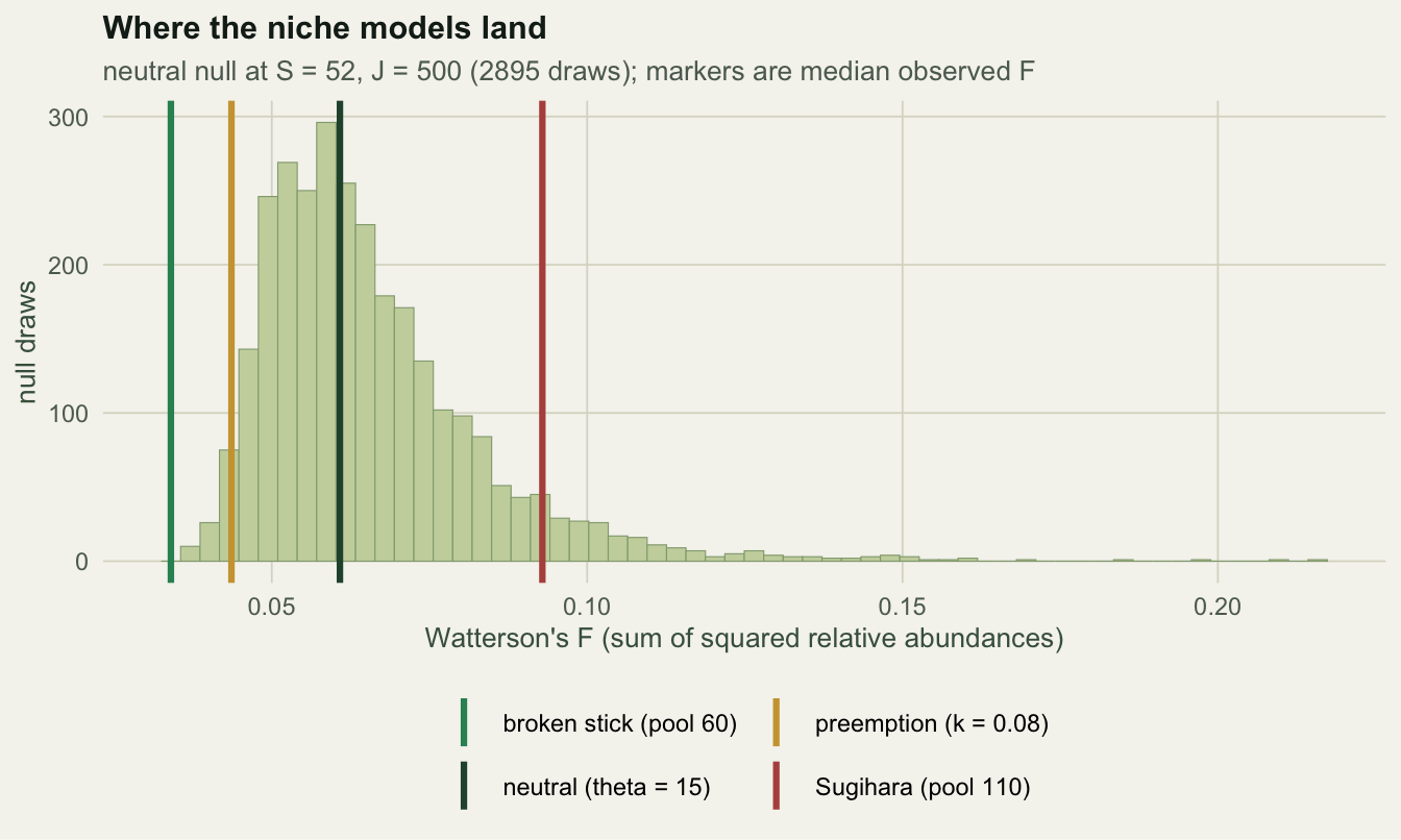
model median_S median_F rejected too_even too_uneven
1 neutral (theta = 15) 54 0.0608 5.2% 3.2% 2.0%
2 broken stick (pool 60) 54 0.0340 93.8% 93.8% 0.0%
3 preemption (k = 0.08) 52 0.0436 52.0% 52.0% 0.0%
4 Sugihara (pool 110) 52 0.0929 31.7% 0.2% 31.5%Read the first row before the rest: on data the null itself generated, the test rejects 5.2% of the time against a nominal 5%. With 500 replicates the Monte Carlo standard error on that figure is 1.0 points, so the test is holding its size, which is what an exactly parameter free null should deliver.
Then three findings, and only one of them is the one you would guess.
The test works, up to a point. Against the broken stick it rejects 93.8% of the time. Against the other two it rejects 52.0% and 31.7%, which means that at a sample size of five hundred individuals, a Sugihara community passes as neutral on roughly two samples in three.
Both tails are in use. The broken stick and the preemption model are rejected for being too even; Sugihara is rejected for being too uneven. A one-sided test built on the assumption that niche structure means dominance would miss two of the three.
The textbook uneven model lands on the even side of neutral. Niche preemption is taught as the geometric series, the model of strong dominance, and here its median \(F\) is 0.0436 against the neutral 0.0608. It is not the evenest generator on the list: the broken stick is, at 0.034. But a model built to produce dominance sitting below neutral at all is the wrong way round, and it is not a quirk of the simulation. It is arithmetic:
p8 <- preemption(300, 0.08)
c(first_species_share = p8[1], F_analytic = sum(p8^2), F_broken_stick_expected = 2 / 61)
first_species_share F_analytic F_broken_stick_expected
0.08000000 0.04166667 0.03278689 To see fifty-odd species in five hundred individuals from a geometric series, the decay constant has to be about 0.08, and a series that decays that slowly is even. Dominance and richness pull against each other, so once you condition on \(S\), the geometric series has nowhere uneven to go.
Does more data help?
The obvious response to 32% power is a bigger plot. It helps, slowly.
J2 <- 2000; Sp2 <- 110                                    # same pool as at J = 500: only J changes
NP2 <- do.call(rbind, lapply(c(10, 15, 22), function(th)
  t(replicate(12000, { x <- sim_esf(th, J2); c(length(x), FF(x)) }))))
colnames(NP2) <- c("S", "F")
q2 <- replicate(300, { x <- draw(sugihara(Sp2), J2); nl <- NP2[NP2[, "S"] == length(x), "F"]
  if (length(nl) < 150) NA else mean(nl <= FF(x)) })
q2 <- q2[!is.na(q2)]
rej2 <- mean(pmin(1, 2 * pmin(q2, 1 - q2)) < 0.05)
data.frame(J = c(J, J2), pool = c(110, Sp2), tested = c(B, length(q2)),
           rejected = c(res$rejected[4], sprintf("%.1f%%", 100 * rej2)))
J pool tested rejected
1 500 110 500 31.7%
2 2000 110 296 35.1%Four times the individuals, drawn from the same pool of 110 species, moves the rejection rate from 31.7% to 35.1%. If your plot is small and your alternative is a niche model like this Sugihara community, the exact test will usually let it through, and that is a property of the data rather than of the test.
Honest limits
Passing is not evidence of neutrality. We measured the failure rate above: one of the three classic alternatives survives this test most of the time at \(J = 500\), and another survives it about half the time. A community that passes has told you that its abundance distribution is not detectably non-Ewens at your sample size, and that sentence is the whole result.
One statistic, one direction each. \(F\) is sensitive to evenness. An alternative that matches the neutral evenness while differing elsewhere, in spatial structure or in which species are common, is invisible to it. Etienne (2007) took a different route for several spatially separated samples from one metacommunity: a new sampling formula, and a test that compares the probability of the observed data with that of data sets simulated from the model at given parameter values. That test is not parameter-free like this one, and it brings spatial information into the null, which is a genuinely different question.
The null is Ewens, not neutrality. The test asks whether the abundances look like a draw from a Dirichlet process. Demographic equivalence implies that; the reverse does not follow. Chave (2004) pointed out that coexistence theories in which species have equal average fitness, including many niche theories, generate the same patterns as neutral theory, and McGill and colleagues (2007) noted that very few abundance distribution models are ever rejected, because few of them predict anything beyond the hollow curve. This test does not fix that. It only removes the part of the problem where the fit was never tested against the data in the first place.
Dispersal limitation is not in this null. Everything here assumes \(m = 1\). A dispersal-limited neutral plot can fail this test, correctly under the Ewens null and misleadingly if you read the failure as evidence against neutral theory. It can also pass, even under strong dispersal limitation: how often it fails depends on \(m\) and \(\theta\). The previous post fits the two-parameter version, and the same conditioning trick does not work there, because \(\theta\) and \(m\) do not factor out.
Where to go next
The exact test checks the abundance shape against the one-parameter null. The next post checks a fitted two-parameter model against its own predictions, which is a different job and turns up a blind spot the two methods share.
References
- Watterson 1978 Genetics 88(2):405-417 (10.1093/genetics/88.2.405)
- Ewens 1972 Theoretical Population Biology 3(1):87-112 (10.1016/0040-5809(72)90035-4)
- Etienne 2007 Ecology Letters 10(7):608-618 (10.1111/j.1461-0248.2007.01052.x)
- MacArthur 1957 PNAS 43(3):293-295 (10.1073/pnas.43.3.293)
- Sugihara 1980 The American Naturalist 116(6):770-787 (10.1086/283669)
- Tokeshi 1990 Journal of Animal Ecology 59(3):1129-1146 (10.2307/5036)
- McGill et al 2007 Ecology Letters 10(10):995-1015 (10.1111/j.1461-0248.2007.01094.x)
- Chave 2004 Ecology Letters 7(3):241-253 (10.1111/j.1461-0248.2003.00566.x)