library(ggplot2)
set.seed(296)Neutral theory in R: theta and the Ewens formula
R
neutral theory
biodiversity
species abundance
ecology tutorial
Fit Hubbell’s fundamental biodiversity number from scratch. The Ewens sampling formula, the exact likelihood, and why species richness is all the data you use.
Corrected 7 October 2026: the post gave the relative bias of the fitted theta in its simulation as if it were the bias of the estimator; it now calls it a simulated value and gives its Monte Carlo standard error beside it.
Hubbell’s neutral theory makes one assumption that everything else follows from: individuals of different species are demographically identical. Same birth rate, same death rate, same dispersal. Species differ only by name. From that starting point the theory predicts an abundance distribution, and the prediction has one free parameter: the fundamental biodiversity number, written \(\theta\).
The theory gets tested by fitting \(\theta\) to an abundance vector and asking how well it fits. This post builds that fit from scratch in base R, and then measures what the fit actually uses. The answer is smaller than most people expect.
Setup
The metacommunity and its urn
The metacommunity is the large, slowly turning species pool. New species enter it by speciation at rate \(\nu\) per birth, and \(\theta = 2 J_M \nu\), where \(J_M\) is the number of individuals in the metacommunity. Keep that definition in view: \(\theta\) is a product. We return to it at the end.
Sampling \(J\) individuals from such a metacommunity has an exact urn description, due to Hoppe. Draw individuals one at a time. Individual \(k+1\) belongs to a species never seen before with probability \(\theta / (\theta + k)\); otherwise it copies the species of one of the \(k\) individuals already drawn, chosen uniformly at random.
sim_esf <- function(theta, J) {
  sp <- integer(J); sp[1] <- 1L; nsp <- 1L
  for (k in 1:(J - 1)) {
    if (runif(1) < theta / (theta + k)) {            # new species
      nsp <- nsp + 1L; sp[k + 1] <- nsp
    } else {                                          # a copy of an existing individual
      sp[k + 1] <- sp[sample.int(k, 1)]
    }
  }
  as.integer(table(sp))
}
sim_esf(theta = 5, J = 20)
[1] 8 2 3 1 1 1 3 1Two lines of R, and no ecology in them at all. That is the point of a neutral model: the species labels do no work.
The Ewens sampling formula
The urn gives a probability for every possible abundance vector. Write \(n_1, \dots, n_S\) for the abundances of the \(S\) species found, \(J = \sum_i n_i\), and \(\Phi_j\) for the number of species represented by exactly \(j\) individuals. Ewens (1972) derived the distribution for population genetics, twenty-nine years before Hubbell wrote it into ecology:
\[P(n_1, \dots, n_S \mid \theta) = \frac{J!}{\prod_{i=1}^{S} n_i \; \prod_{j=1}^{J} \Phi_j!} \cdot \frac{\theta^S}{(\theta)_J}\]
where \((\theta)_J = \theta(\theta+1)\cdots(\theta+J-1)\) is the rising factorial. In R, on the log scale:
lpoch <- function(x, n) if (n == 0) 0 else sum(log(x + 0:(n - 1)))   # rising factorial

esf_loglik <- function(n, theta) {
  J <- sum(n); S <- length(n)
  phi <- as.numeric(table(n))
  const <- lfactorial(J) - sum(log(n)) - sum(lfactorial(phi))
  const + S * log(theta) - lpoch(theta, J)
}
Before trusting it, check that it is a probability distribution. For a sample of six individuals there are eleven possible abundance vectors, so we can enumerate all of them and add the probabilities up.
parts <- function(J, mx = J) {
  if (J == 0) return(list(integer(0)))
  out <- list()
  for (k in min(J, mx):1) for (p in parts(J - k, k)) out[[length(out) + 1]] <- c(k, p)
  out
}
P6 <- parts(6)
tot <- sapply(c(0.5, 2, 10), function(th) sum(sapply(P6, function(n) exp(esf_loglik(n, th)))))
n_p6 <- length(P6)
signif(tot, 12)
[1] 1 1 1Three values of \(\theta\), three sums of exactly one. The formula is correctly normalised over the 11 partitions of six.
What the fit uses
Look again at the formula. It has two factors. The first one, the combinatorial constant, contains every abundance in the sample. The second one, \(\theta^S / (\theta)_J\), is the only place \(\theta\) appears, and it contains only \(S\) and \(J\).
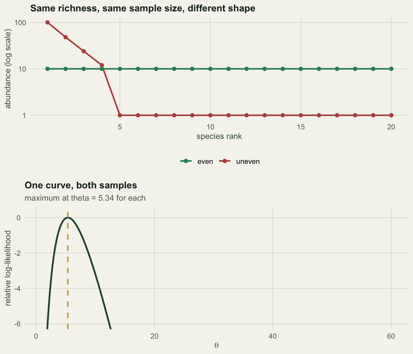
That is a sufficiency statement, and it has a consequence you can measure. Take two samples of 200 individuals holding 20 species each. Make one of them as even as arithmetic allows and the other as lopsided as we like.
J <- 200
even   <- rep(10L, 20)                                  # every species 10 individuals
uneven <- c(100L, 48L, 24L, 12L, rep(1L, 16))           # one species is half the sample
c(J_even = sum(even), S_even = length(even), J_uneven = sum(uneven), S_uneven = length(uneven))
J_even S_even J_uneven S_uneven
200 20 200 20 simpson <- function(n) 1 - sum((n / sum(n))^2)
ev_simp <- simpson(even); un_simp <- simpson(uneven)
round(c(Simpson_even = ev_simp, Simpson_uneven = un_simp,
dominance_even = max(even) / J, dominance_uneven = max(uneven) / J), 3) Simpson_even Simpson_uneven dominance_even dominance_uneven
0.950 0.674 0.050 0.500 One sample has a dominant species holding 50% of the individuals; the other has no species above 5%. By eye they are different communities. Now fit \(\theta\) to each. The maximum likelihood estimate solves a single equation: set the expected richness equal to the observed richness. The expectation has a closed form, \(\mathrm{E}[S] = \theta(\psi(\theta + J) - \psi(\theta))\), with \(\psi\) the digamma function.
ES <- function(theta, J) theta * (digamma(theta + J) - digamma(theta))
theta_mle <- function(S, J) uniroot(function(th) ES(th, J) - S, c(1e-8, 1e6), tol = 1e-10)$root

th_even   <- theta_mle(length(even),   sum(even))
th_uneven <- theta_mle(length(uneven), sum(uneven))
c(theta_even = th_even, theta_uneven = th_uneven, difference = abs(th_even - th_uneven))
theta_even theta_uneven difference
5.343537 5.343537 0.000000 The two estimates are not merely close. The difference between them is 0, exactly, and that is not a coincidence of these two vectors: the entire log-likelihood gap between them is a constant that does not move with \(\theta\).
grid <- seq(1, 60, length.out = 400)
gap  <- sapply(grid, function(x) esf_loglik(even, x) - esf_loglik(uneven, x))
gap_sd <- sd(gap)
sci_tex <- function(x, d = 1) {                       # readable exponent form for the prose
  e <- floor(log10(abs(x))); sprintf("$%.*f \\times 10^{%d}$", d, x / 10^e, e)
}
c(min_gap = min(gap), max_gap = max(gap), sd_gap = gap_sd)
min_gap max_gap sd_gap
-4.357613e+01 -4.357613e+01 3.461980e-14 Across four hundred values of \(\theta\) the gap varies by \(3.5 \times 10^{-14}\), which is floating point noise. The abundances shift the likelihood up or down by a fixed amount and then say nothing further. Fitting Hubbell’s \(\theta\) to a species abundance distribution is fitting it to one number.
Is the estimator any good?
Sufficiency is not accuracy. Simulate two thousand samples from the urn at a known \(\theta\), fit each one, and look at the sampling distribution. The interval comes from the profile likelihood, which for a one-parameter fit is the whole likelihood.
theta_ci <- function(S, J) {
  part <- function(x) S * log(x) - lpoch(x, J)
  th <- theta_mle(S, J); mx <- part(th)
  f <- function(x) part(x) - mx + qchisq(0.95, 1) / 2
  c(uniroot(f, c(1e-6, th))$root, uniroot(f, c(th, 1e5))$root)
}
th_true <- 5.5; B <- 2000
mc <- t(replicate(B, {
  x <- sim_esf(th_true, J); S <- length(x)
  c(theta_mle(S, J), theta_ci(S, J))
}))
cal_mean <- mean(mc[, 1]); cal_med <- median(mc[, 1])
cal_cov  <- mean(mc[, 2] <= th_true & mc[, 3] >= th_true)
round(c(true = th_true, mean_est = cal_mean, median_est = cal_med, coverage = cal_cov), 3)
true mean_est median_est coverage
5.500 5.522 5.344 0.949 Mean estimate 5.52 against a true 5.5, a simulated relative bias of +0.4% with a Monte Carlo standard error of 0.6%, and interval coverage 0.949 against a nominal 0.95. The estimator does what it says. Applied to our worked pair, the interval is:
ci20 <- theta_ci(20, 200)
round(c(lower = ci20[1], mle = th_even, upper = ci20[2]), 2)
lower mle upper
3.08 5.34 8.74 Both samples, one interval, because both samples have \(S = 20\) and \(J = 200\).
Where Fisher’s log-series comes from
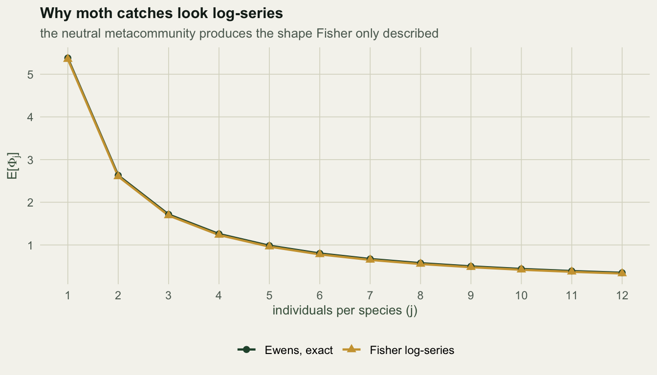
The Ewens formula also settles an old question. Fisher, Corbet and Williams (1943) fitted a log-series to butterfly and moth catches, and Fisher derived it as a limiting form of the negative binomial from an assumed gamma distribution of abundances, with no biological mechanism behind that assumption. The neutral metacommunity supplies one. The expected number of species with exactly \(j\) individuals under the Ewens formula is
\[\mathrm{E}[\Phi_j] = \frac{\theta}{j}\cdot\frac{J!}{(J-j)!}\cdot\frac{\Gamma(\theta + J - j)}{\Gamma(\theta + J)}\]
and for \(j\) well below \(J\) this collapses to \(\theta x^j / j\) with \(x = J / (\theta + J)\), which is Fisher’s log-series with \(\alpha = \theta\).
Ephi <- function(theta, J, j) exp(log(theta) - log(j) + lfactorial(J) - lfactorial(J - j) +
                                    lgamma(theta + J - j) - lgamma(theta + J))
lser <- function(theta, J, j) theta * (J / (theta + J))^j / j
jj <- 1:12
cmp <- data.frame(j = jj, exact = Ephi(5.5, 200, jj), log_series = lser(5.5, 200, jj))
cmp$pct_gap <- 100 * (cmp$log_series / cmp$exact - 1)
sum_phi <- sum(Ephi(5.5, 200, 1:200)); es55 <- ES(5.5, 200)
round(cmp, 4)
j exact log_series pct_gap
1 1 5.3790 5.3528 -0.4866
2 2 2.6300 2.6048 -0.9599
3 3 1.7144 1.6900 -1.4200
4 4 1.2571 1.2336 -1.8668
5 5 0.9831 0.9605 -2.3005
6 6 0.8008 0.7790 -2.7210
7 7 0.6708 0.6498 -3.1285
8 8 0.5736 0.5534 -3.5230
9 9 0.4982 0.4787 -3.9044
10 10 0.4380 0.4193 -4.2729
11 11 0.3890 0.3710 -4.6284
12 12 0.3483 0.3310 -4.9709The two agree to 0.5% at singletons and drift apart to 5.0% by twelve individuals, because the log-series ignores the fact that the sample is finite. And the expected counts add up to the expected richness, 20.4155 against 20.4155, which is a useful check that the two formulas describe one model.
What theta is not
Two limits are worth stating plainly, because the literature is not always plain about them.
Theta is a product. The definition is \(\theta = 2 J_M \nu\), and the likelihood is a function of \(\theta\) and nothing else. So our fitted value is consistent with any metacommunity size at all, provided the speciation rate moves to compensate:
JM <- c(1e6, 1e9, 1e12)
data.frame(J_M = format(JM, scientific = TRUE),
           nu_implied = signif(th_even / (2 * JM), 3),
           theta = th_even / (2 * JM) * 2 * JM)
J_M nu_implied theta
1 1e+06 2.67e-06 5.343537
2 1e+09 2.67e-09 5.343537
3 1e+12 2.67e-12 5.343537Six orders of magnitude in the speciation rate, one likelihood. No quantity of abundance data separates the size of the species pool from the rate at which species enter it. When a paper reports a fitted speciation rate, it is reporting an assumed \(J_M\).
The fit uses one number. We measured that above. A rank abundance curve drawn through a fitted neutral prediction looks like a model being tested against a shape, but the shape had no vote. This does not make the fit wrong; it makes the apparent agreement much weaker evidence than it looks. Two ways out exist, and both have their own post: allow dispersal limitation, which gives the abundances something to say, or test the shape directly with a statistic that conditions on \(S\).
The sample is a snapshot. The neutral theory is a claim about dynamics: drift, speciation, dispersal. An abundance vector taken once carries no information about turnover rates. Nothing above tests demographic equivalence; it tests one distributional consequence of it.
Where to go next
The obvious follow-up is to relax the assumption that your plot is a random draw from the metacommunity, which is what the next post does. If your interest is the fitting of abundance distributions in general rather than the neutral theory in particular, the species abundance distribution post covers the descriptive families, and the diversity estimation posts cover what the unseen species do to any of this.
References
- Ewens 1972 Theoretical Population Biology 3(1):87-112 (10.1016/0040-5809(72)90035-4)
- Fisher, Corbet & Williams 1943 Journal of Animal Ecology 12(1):42-58 (10.2307/1411)
- Hubbell 2001 The Unified Neutral Theory of Biodiversity and Biogeography, ISBN 978-0-691-02128-7
- Chave 2004 Ecology Letters 7(3):241-253 (10.1111/j.1461-0248.2003.00566.x)
- Alonso & McKane 2004 Ecology Letters 7(10):901-910 (10.1111/j.1461-0248.2004.00640.x)
- Rosindell, Hubbell & Etienne 2011 Trends in Ecology and Evolution 26(7):340-348 (10.1016/j.tree.2011.03.024)