library(ggplot2)
set.seed(297)Dispersal limitation: fitting theta and m in R
R
neutral theory
biodiversity
dispersal
likelihood
ecology tutorial
Etienne’s sampling formula in base R. Why fitting Ewens to a dispersal-limited plot can underestimate theta by two thirds, and how immigration fixes most of it.
Corrected 15 October 2026: a sentence on the limits of the correction still presented it as recovering theta and m on data the model generated, and the description said immigration repairs the underestimate; both now say it removes most of the bias. The description also stated the naive fit’s underestimate of two thirds as general; it now says the naive fit can underestimate theta that much.
Corrected 7 October 2026: the post said Etienne’s formula recovers theta and m; it now says it removes most of the bias but leaves the median estimate of theta below the truth and that of m above it. It also said that the boundary case, where the estimate of theta runs off to infinity, is not rare; it now says that the checking post finds such estimates rare, although intervals with no upper limit are common there.
Corrected 30 September 2026: the Etienne fits started the optimiser from a single point, which on some plots stopped on the lower of two likelihood peaks. They now keep the best of several starts, which lowers the median estimate of theta, strengthens the theta-m trade-off and moves the cross in the ridge figure to the higher peak. The closing section also said Etienne, Alonso and McKane showed that several structural assumptions can be relaxed without changing the sampling formula; it now says their result concerns the zero-sum assumption.
The previous post fitted Hubbell’s \(\theta\) with the Ewens sampling formula, and the formula assumes your plot is a random draw from the metacommunity. Every individual in your quadrat arrived independently from the whole species pool.
No real plot works like that. A seed that lands under its parent is not a random draw from anything. That gap has a name in the theory, dispersal limitation, and a parameter, the immigration probability \(m\). This post fits \(\theta\) and \(m\) together, and measures what happens if you do not.
Setup
The local community
Hubbell’s local community is a second urn sitting downstream of the first. Fill a plot of \(J\) individuals one at a time. Each new individual is an immigrant from the metacommunity with probability \(m\), and otherwise a copy of an individual already in the plot. Immigrants carry metacommunity species labels, so the metacommunity urn from the previous post supplies them.
It is more convenient to work with the fundamental dispersal number \(I\), which relates to \(m\) by \(I = m(J-1)/(1-m)\). The reason for the reparameterisation is that \(I\) plays exactly the role \(\theta\) plays one level up: at step \(k\), the next individual is an immigrant with probability \(I/(I+k)\).
sim_etienne <- function(theta, I, J) {
  loc <- integer(J); anc <- integer(0); nsp <- 0L
  for (k in 0:(J - 1)) {
    if (runif(1) < I / (I + k)) {                       # immigration event
      A <- length(anc)
      if (A == 0 || runif(1) < theta / (theta + A)) {   # the immigrant is a new species
        nsp <- nsp + 1L; s <- nsp
      } else {                                          # the species of an earlier immigrant
        s <- anc[sample.int(A, 1)]
      }
      anc <- c(anc, s); loc[k + 1] <- s
    } else {                                            # local reproduction
      loc[k + 1] <- loc[sample.int(k, 1)]
    }
  }
  as.integer(table(loc))
}
m_to_I <- function(m, J) m * (J - 1) / (1 - m)
I_to_m <- function(I, J) I / (I + J - 1)
The nesting is what makes the model work: the plot samples \(A\) immigration events from the metacommunity, and those \(A\) ancestors are an Ewens sample. Since the immigration urn has the same structure as the Hoppe urn, the expected number of immigration events reuses the digamma formula from the previous post.
ES <- function(theta, J) theta * (digamma(theta + J) - digamma(theta))
theta_true <- 50; m_true <- 0.05; J <- 1000
I_true <- m_to_I(m_true, J)
EA <- ES(I_true, J)                                     # expected number of immigration events
c(I = I_true, E_immigration_events = EA, E_S_from_those_events = ES(theta_true, EA),
  E_S_if_m_were_1 = ES(theta_true, J))
I E_immigration_events E_S_from_those_events
52.57895 158.03903 71.66654
E_S_if_m_were_1
152.70398 The last two numbers are the whole problem. A thousand individuals drawn straight from the metacommunity would hold about 153 species. The same thousand individuals with five per cent immigration hold about 72, because they descend from only about 158 independent arrivals. Dispersal limitation does not just reshape the abundance curve, it destroys most of the richness.
What Ewens does with such a plot
The previous post showed that the Ewens fit reads \(S\) and \(J\) and nothing else. Feed it a dispersal-limited plot and it sees a poor, apparently species-starved sample, and reports the only \(\theta\) that could produce it under \(m = 1\).
theta_mle <- function(S, J) {
  if (S <= 1 || S >= J) return(NA_real_)
  uniroot(function(th) ES(th, J) - S, c(1e-8, 1e6), tol = 1e-10)$root
}
d1 <- sort(sim_etienne(theta_true, I_true, J), decreasing = TRUE)
c(S_observed = length(d1), J = sum(d1), theta_naive = theta_mle(length(d1), J), theta_true = theta_true)
S_observed J theta_naive theta_true
69.00000 1000.00000 16.66303 50.00000 One sample proves nothing, so we repeat it later. First we need the correction.
Etienne’s sampling formula
Etienne (2005) marginalised the unobserved number of immigration events out of the likelihood, the same move that makes an N-mixture or an occupancy model work. Conditional on \(A\) ancestors, the plot is a known combinatorial object; sum over all \(A\) from \(S\) to \(J\):
\[P(D \mid \theta, I) = \frac{J!}{\prod_i n_i \prod_j \Phi_j!} \cdot \frac{1}{(I)_J} \sum_{A=S}^{J} K(D, A) \, \frac{\theta^S}{(\theta)_A} \, I^A\]
The weights \(K(D,A)\) are the awkward part. They count the ways the observed abundances can descend from \(A\) ancestors, they depend only on the data, and they are built from unsigned Stirling numbers of the first kind. Because they do not involve \(\theta\) or \(I\), you compute them once and reuse them at every step of the optimiser.
log_stirling1 <- function(N) {                          # log |s(n,k)|, n = 0..N
  L <- matrix(-Inf, N + 1, N + 1); L[1, 1] <- 0
  for (n in 0:(N - 1)) for (k in 0:(n + 1)) {
    a <- if (k >= 1) L[n + 1, k] else -Inf
    b <- if (n >= 1) log(n) + L[n + 1, k + 1] else -Inf
    mx <- max(a, b)
    L[n + 2, k + 1] <- if (is.infinite(mx)) -Inf else mx + log(exp(a - mx) + exp(b - mx))
  }
  L
}
LS5 <- log_stirling1(5)
round(exp(LS5[6, 2:6]))                                 # s(5,k), k = 1..5
[1] 24 50 35 10 1Those are 24, 50, 35, 10, 1, and they sum to 120, which is \(5!\), as unsigned Stirling numbers of the first kind must.
A trap worth knowing about
\(K(D, \cdot)\) is a convolution of per-species vectors, and R ships a fast convolution in stats::convolve. Using it here is a mistake. The terms being convolved span many orders of magnitude, and convolve works through the FFT, whose round-off is relative to the largest term in the transform. The small entries come back as noise, and some come back negative. Write the direct version instead; it is a few lines and it is fast enough.
conv_direct <- function(a, b) {
  if (length(a) > length(b)) { tmp <- a; a <- b; b <- tmp }   # loop over the shorter vector
  r <- numeric(length(a) + length(b) - 1)
  for (i in seq_along(a)) r[i + seq_along(b) - 1] <- r[i + seq_along(b) - 1] + a[i] * b
  r
}
logK <- function(n, LS) {
  S <- length(n); Jn <- sum(n)
  cur <- 1; off <- 0
  for (i in seq_len(S)) {
    a  <- 1:n[i]
    lv <- LS[n[i] + 1, a + 1] + lgamma(a) - lgamma(n[i])      # log s(n_i,a) + log(a-1)! - log(n_i-1)!
    M  <- max(lv); off <- off + M
    cur <- conv_direct(cur, exp(lv - M))
    m2 <- max(cur); cur <- cur / m2; off <- off + log(m2)     # renormalised at each step
  }
  out <- rep(-Inf, Jn + 1)                                    # index: A + 1
  out[(S:Jn) + 1] <- log(pmax(cur[(S:Jn) - S + 1], 0)) + off
  out
}
The identity that catches the FFT version is exact and costs nothing to check: \(K(D, S) = K(D, J) = 1\) for any \(D\), because there is exactly one way for the sample to descend from \(S\) ancestors (one per species) and exactly one way for it to descend from \(J\) (one per individual).
LK1 <- logK(d1, log_stirling1(max(d1)))
c(K_at_S = exp(LK1[length(d1) + 1]), K_at_J = exp(LK1[J + 1]))
K_at_S K_at_J
1 1 Now the likelihood itself.
lpoch <- function(x, n) if (n == 0) 0 else sum(log(x + 0:(n - 1)))
sci_tex <- function(x, d = 1) {                         # readable exponent form for the prose
  e <- floor(log10(abs(x))); sprintf("$%.*f \\times 10^{%d}$", d, x / 10^e, e)
}
etienne_loglik <- function(n, theta, I, LK) {
  Jn <- sum(n); S <- length(n)
  const <- lfactorial(Jn) - sum(log(n)) - sum(lfactorial(as.numeric(table(n))))
  A   <- S:Jn
  lpt <- cumsum(log(theta + 0:(Jn - 1)))                # (theta)_A for every A, in one pass
  tt  <- LK[A + 1] + S * log(theta) - lpt[A] + A * log(I)
  mx  <- max(tt)
  const + mx + log(sum(exp(tt - mx))) - lpoch(I, Jn)    # log-sum-exp
}
fit_etienne <- function(n) {
  Jn <- sum(n); LK <- logK(n, log_stirling1(max(n)))    # ONCE, before the optimisation
  nll <- function(p) -etienne_loglik(n, exp(p[1]), exp(p[2]), LK)
  starts <- expand.grid(log(c(5, 20, 80, 400)), log(c(5, 20, 80, 400)))   # the ridge can hold two peaks
  fits <- lapply(seq_len(nrow(starts)), function(i)
    optim(unname(unlist(starts[i, ])), nll, method = "Nelder-Mead", control = list(reltol = 1e-12, maxit = 3000)))
  f <- fits[[which.min(sapply(fits, `[[`, "value"))]]                    # keep the best of sixteen starts
  list(theta = exp(f$par[1]), I = exp(f$par[2]), m = I_to_m(exp(f$par[2]), Jn), logL = -f$value)
}
Two checks before it is allowed near data. The formula must be a probability distribution, so enumerate all abundance vectors for a small \(J\) and add them up. And as \(I\) grows, every individual becomes an immigrant, \(m\) approaches one, and the formula must collapse back to Ewens.
parts <- function(Jn, mx = Jn) {
  if (Jn == 0) return(list(integer(0)))
  out <- list(); for (k in min(Jn, mx):1) for (p in parts(Jn - k, k)) out[[length(out) + 1]] <- c(k, p)
  out
}
P6 <- parts(6)
tot6 <- sapply(list(c(3, 8), c(20, 2)), function(pr)
  sum(sapply(P6, function(n) exp(etienne_loglik(n, pr[1], pr[2], logK(n, log_stirling1(max(n))))))))
esf_loglik <- function(n, theta) {
  const <- lfactorial(sum(n)) - sum(log(n)) - sum(lfactorial(as.numeric(table(n))))
  const + length(n) * log(theta) - lpoch(theta, sum(n))
}
dsm <- c(4, 2, 2, 1, 1)
lim <- sapply(10^(3:9), function(Ibig)
  etienne_loglik(dsm, 6, Ibig, logK(dsm, log_stirling1(max(dsm)))) - esf_loglik(dsm, 6))
data.frame(I = 10^(3:9), gap_vs_Ewens = signif(lim, 3), gap_times_I = signif(lim * 10^(3:9), 3))
I gap_vs_Ewens gap_times_I
1 1e+03 1.48e-02 14.8
2 1e+04 1.50e-03 15.0
3 1e+05 1.50e-04 15.0
4 1e+06 1.50e-05 15.0
5 1e+07 1.50e-06 15.0
6 1e+08 1.50e-07 15.0
7 1e+09 1.50e-08 15.0Both sums are 1. And the gap to the Ewens likelihood shrinks exactly in proportion to \(1/I\): multiplying the gap by \(I\) gives a constant, 15.0, holding from \(I = 10^4\) up to \(I = 10^9\). That is the behaviour a correct nesting must show, and it is the kind of check an FFT-based logK fails loudly.
The measurement
Simulate three hundred plots at a known \(\theta\) and \(m\), fit each one both ways, and compare.
B <- 300
mc <- t(replicate(B, {
  d <- sort(sim_etienne(theta_true, I_true, J), decreasing = TRUE)
  f <- fit_etienne(d)
  c(theta_naive = theta_mle(length(d), J), theta_et = f$theta, m_et = f$m, S = length(d))
}))
q <- function(x) c(median = median(x), lo = unname(quantile(x, 0.05)), hi = unname(quantile(x, 0.95)))
round(rbind(theta_naive = q(mc[, "theta_naive"]), theta_etienne = q(mc[, "theta_et"]),
            m_etienne = q(mc[, "m_et"]), S_observed = q(mc[, "S"])), 4)
median lo hi
theta_naive 17.3065 14.1655 20.9800
theta_etienne 43.5990 20.5033 150.8375
m_etienne 0.0581 0.0228 0.3966
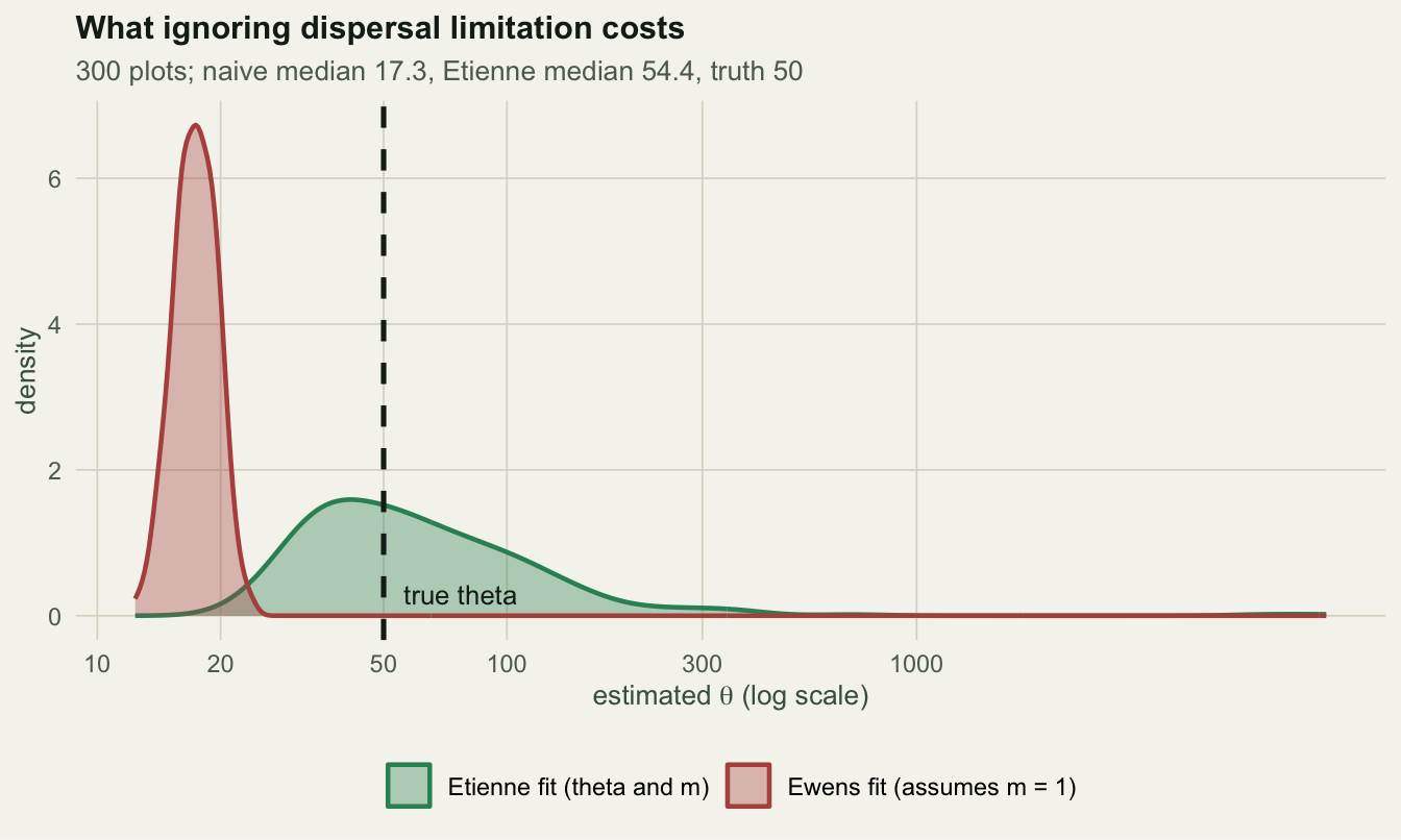
S_observed 71.0000 61.0000 82.0000The naive Ewens fit reports a median \(\theta\) of 17.3 against a true 50, an error of -65%. It is not noisy, it is wrong in a fixed direction: 100% of the three hundred estimates land below the truth. Etienne’s formula gives medians of 43.6 for \(\theta\) and 0.0581 for \(m\), against 50 and 0.05: most of the bias is gone, though the median of \(\hat\theta\) still sits below the truth and that of \(\hat m\) above it.
The abundances now matter, and one of them refuses to answer
One consequence is worth checking directly. Under Ewens, the two samples from the previous post gave identical fits because both had \(S = 20\) and \(J = 200\). Under Etienne they do not.
even   <- rep(10L, 20)
uneven <- c(100L, 48L, 24L, 12L, rep(1L, 16))
fe <- fit_etienne(sort(even, decreasing = TRUE))
fu <- fit_etienne(sort(uneven, decreasing = TRUE))
rbind(even   = c(theta = fe$theta, I = fe$I, m = fe$m, logL = fe$logL),
      uneven = c(theta = fu$theta, I = fu$I, m = fu$m, logL = fu$logL))
theta I m logL
even 10.315991 2.757715e+01 0.121712 -68.77381
uneven 5.343538 1.704496e+14 1.000000 -30.65623The even sample gets a sensible interior fit. The uneven one sends \(\theta\) to \(5.3 \times 10^{0}\), which looks like an optimiser that lost its footing. It is not. It is an exact limit of the formula, and the formula is telling us something.
Look at the sum over \(A\). Each term carries \(\theta^S / (\theta)_A\), and for large \(\theta\) the rising factorial behaves like \(\theta^A\), so the term scales as \(\theta^{S-A}\). Every \(A\) above \(S\) is crushed. Only \(A = S\) survives, where \(K(D,S) = 1\), and what is left is
\[\lim_{\theta \to \infty} P(D \mid \theta, I) = \frac{J!}{\prod_i n_i \prod_j \Phi_j!} \cdot \frac{I^S}{(I)_J}\]
which is the Ewens sampling formula with \(I\) in place of \(\theta\). An infinitely diverse metacommunity makes every immigrant a new species, the two levels collapse into one, and the immigration number takes over the role the biodiversity number played.
theta_grid <- 10^(2:12)
gap <- sapply(theta_grid, function(th) etienne_loglik(uneven, th, 5, LK = logK(uneven, log_stirling1(max(uneven)))) -
                esf_loglik(uneven, 5))
th_ew <- theta_mle(length(uneven), sum(uneven))
c(gap_at_theta_1e12 = gap[11], I_hat_uneven = fu$I, theta_Ewens_uneven = th_ew,
  difference = abs(fu$I - th_ew), logL_gap = abs(fu$logL - esf_loglik(uneven, th_ew)))
gap_at_theta_1e12 I_hat_uneven theta_Ewens_uneven difference
-1.080025e-10 1.704496e+14 5.343537e+00 1.704496e+14
logL_gap
9.094947e-13 The check is exact twice over. The Etienne likelihood at \(\theta = 10^{12}\) sits \(1.1 \times 10^{-10}\) from the Ewens likelihood at \(I\), and the fitted \(\hat I\) for the uneven sample equals its Ewens \(\hat\theta\) to \(1.7 \times 10^{14}\), with log-likelihoods agreeing to \(9.1 \times 10^{-13}\). The two fits are the same fit.
So the abundance shape did get a vote, and on the uneven sample the vote was a refusal. The profile likelihood makes the refusal visible: it climbs, flattens, and never turns back.
LKu <- logK(uneven, log_stirling1(max(uneven)))
prof <- sapply(10^(1:8), function(th)
  -optimize(function(li) -etienne_loglik(uneven, th, exp(li), LK = LKu), c(log(0.2), log(4000)))$objective)
data.frame(theta = 10^(1:8), profile_logL = round(prof, 3))
theta profile_logL
1 1e+01 -34.026
2 1e+02 -31.629
3 1e+03 -30.758
4 1e+04 -30.666
5 1e+05 -30.657
6 1e+06 -30.656
7 1e+07 -30.656
8 1e+08 -30.656Read that as an ecological statement rather than a numerical one. The best explanation of a plot with one species holding half the individuals and sixteen singletons is: twenty species arrived as twenty separate immigrants, and local reproduction did everything after that. Nothing in the sample bounds how diverse the source pool was, so nothing bounds \(\theta\). The even sample, by contrast, does bound it, and beats the one-parameter Ewens fit by 5.5 log units.
The checking post measures how often this happens on data the model generated itself: an interval for \(\theta\) with no upper limit is common there, but an estimate that runs off to infinity, as here, is rare.
Honest limits
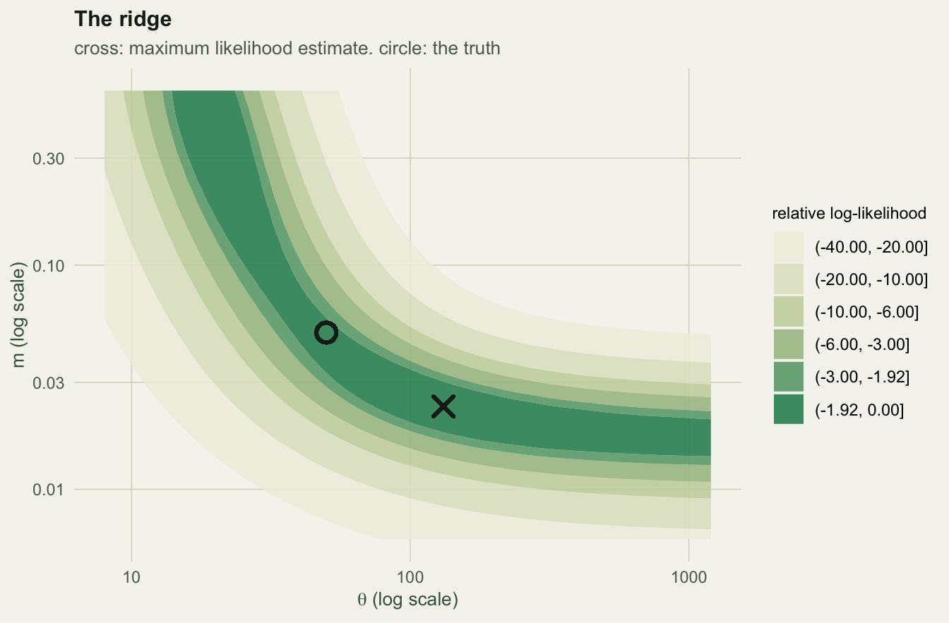
Theta and m trade off. Across the three hundred simulated plots, the two estimates are negatively correlated on the log scale, -0.84. The likelihood has a ridge: a plot that looks species-poor can be explained by a small metacommunity or by a plot that rarely receives immigrants, and the data separate the two weakly. The ridge can also carry two separate peaks, one at small \(\theta\) and large \(m\) and one at large \(\theta\) and small \(m\), which is why fit_etienne starts the optimiser from a grid of points and keeps the best: a single start can stop on the lower peak, as it does from several starting points for the plot in the figure below. The ninety-fifth percentile of \(\hat\theta\) sits at 151, 3.0 times the truth, on data generated by the model itself.
The correction is not a licence. Removing most of the bias on data the model generated, as Etienne’s formula does here, is the minimum a fitting routine must do, not evidence that a real plot is neutral. Etienne, Alonso and McKane (2007) showed that the zero-sum constraint can be dropped without changing the sampling formula of a community at equilibrium, which means fitting the formula well says nothing about that assumption and tests less of the theory than the derivation suggests.
Two parameters, one snapshot. \(m\) is a per-birth immigration probability, estimated from a single census with no dispersal data in it. It absorbs anything that makes a plot more aggregated than a random metacommunity draw: clonal growth, seed shadow, a patch of favourable soil, or a competitor holding a site. Only the seed shadow is dispersal.
Where to go next
Fitting the model is the easy half. The next two posts do the harder half: a test of whether the abundance shape is neutral at all, and a set of checks on the fit itself.
References
- Etienne 2005 Ecology Letters 8(3):253-260 (10.1111/j.1461-0248.2004.00717.x)
- Etienne & Alonso 2005 Ecology Letters 8(11):1147-1156 (10.1111/j.1461-0248.2005.00817.x)
- Etienne, Alonso & McKane 2007 Journal of Theoretical Biology 248(3):522-536 (10.1016/j.jtbi.2007.06.010)
- Alonso & McKane 2004 Ecology Letters 7(10):901-910 (10.1111/j.1461-0248.2004.00640.x)
- Hubbell 2001 The Unified Neutral Theory of Biodiversity and Biogeography, ISBN 978-0-691-02128-7
- Rosindell, Hubbell & Etienne 2011 Trends in Ecology and Evolution 26(7):340-348 (10.1016/j.tree.2011.03.024)