library(ggplot2)
set.seed(299)Checking a neutral model fit
R
neutral theory
model checking
likelihood
ecology tutorial
Three checks on a fitted neutral model in R: interval calibration, out-of-sample richness prediction on nested subsamples, and what stays unidentifiable.
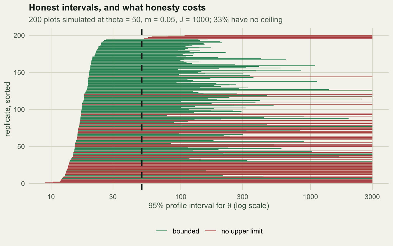
Corrected 7 October 2026: check one said the interval covers the truth so often partly because many intervals have no upper limit, each from a profile that never comes back down; it now shows that the open-ended intervals cover the truth less often than the bounded ones and that all but one of them peak and then fall back by less than the cut, and the figure caption now mentions the bounded intervals clipped at its edge. Check two now computes the calibrated band behind the statement that most Sugihara communities pass the nested check, and the post no longer says that the two checks are not independent tests or that a further check of the same shape would add nothing, since it never runs them on the same samples.
Corrected 1 October 2026: the post said that the nested-subsample check never catches the Sugihara community with a pool of eighty and that the two checks are one test run twice; it now says that the nested check lets that community through about as often as the exact test does, and that both let it through most of the time.
Corrected 30 September 2026: the calibration check fitted each simulated plot from a single starting point, which on some plots stopped on a lower peak of the likelihood. The fits now keep the best of a grid of starts, which moves the median estimate of theta from just above the truth to a little below it and changes the coverage and the share of intervals with no upper limit slightly.
The previous two posts fit Hubbell’s model and tested its abundance prediction. This one asks what the fit is worth once you have it. Three checks, in the order that finds problems fastest: does the interval mean what it says, does the fitted model predict anything it was not shown, and what does the likelihood refuse to identify no matter how much data you collect.
The pattern generalises past neutral theory. The checks are cheap, they are all Monte Carlo, and each one has to be run on data where it should fail as well as data where it should pass. A check that cannot fail is not a check.
Setup
The machinery is from the previous two posts, compressed. The Ewens side needs one root find; the Etienne side needs Stirling numbers and a convolution.
ES <- function(theta, J) theta * (digamma(theta + J) - digamma(theta))
theta_mle <- function(S, J) {
  if (S <= 1 || S >= J) return(NA_real_)
  uniroot(function(th) ES(th, J) - S, c(1e-8, 1e6), tol = 1e-10)$root
}
lpoch <- function(x, n) if (n == 0) 0 else sum(log(x + 0:(n - 1)))
log_stirling1 <- function(N) {
  L <- matrix(-Inf, N + 1, N + 1); L[1, 1] <- 0
  for (n in 0:(N - 1)) for (k in 0:(n + 1)) {
    a <- if (k >= 1) L[n + 1, k] else -Inf
    b <- if (n >= 1) log(n) + L[n + 1, k + 1] else -Inf
    mx <- max(a, b)
    L[n + 2, k + 1] <- if (is.infinite(mx)) -Inf else mx + log(exp(a - mx) + exp(b - mx))
  }
  L
}
conv_direct <- function(a, b) {
  if (length(a) > length(b)) { tmp <- a; a <- b; b <- tmp }
  r <- numeric(length(a) + length(b) - 1)
  for (i in seq_along(a)) r[i + seq_along(b) - 1] <- r[i + seq_along(b) - 1] + a[i] * b
  r
}
logK <- function(n, LS) {
  S <- length(n); Jn <- sum(n); cur <- 1; off <- 0
  for (i in seq_len(S)) {
    a <- 1:n[i]
    lv <- LS[n[i] + 1, a + 1] + lgamma(a) - lgamma(n[i])
    M <- max(lv); off <- off + M
    cur <- conv_direct(cur, exp(lv - M))
    m2 <- max(cur); cur <- cur / m2; off <- off + log(m2)
  }
  out <- rep(-Inf, Jn + 1); out[(S:Jn) + 1] <- log(pmax(cur[(S:Jn) - S + 1], 0)) + off; out
}
etienne_loglik <- function(n, theta, I, LK) {
  Jn <- sum(n); S <- length(n)
  const <- lfactorial(Jn) - sum(log(n)) - sum(lfactorial(as.numeric(table(n))))
  A <- S:Jn; lpt <- cumsum(log(theta + 0:(Jn - 1)))
  tt <- LK[A + 1] + S * log(theta) - lpt[A] + A * log(I)
  mx <- max(tt); const + mx + log(sum(exp(tt - mx))) - lpoch(I, Jn)
}
sim_etienne <- function(theta, I, J) {
  loc <- integer(J); anc <- integer(0); ns <- 0L
  for (k in 0:(J - 1)) {
    if (runif(1) < I / (I + k)) {
      A <- length(anc)
      if (A == 0 || runif(1) < theta / (theta + A)) { ns <- ns + 1L; s <- ns } else s <- anc[sample.int(A, 1)]
      anc <- c(anc, s); loc[k + 1] <- s
    } else loc[k + 1] <- loc[sample.int(k, 1)]
  }
  as.integer(table(loc))
}
m_to_I <- function(m, J) m * (J - 1) / (1 - m)
Check one: does the interval mean what it says
A confidence interval that covers the truth 95% of the time is doing its job. The only way to know is to generate data from the model at a known parameter and count. Fit each simulated plot (from a grid of starting points, since the likelihood can have more than one peak and a single start can stop on the lower one), then invert the profile likelihood.
fit2 <- function(n, LK) {
  Jn <- sum(n)
  nll <- function(p) -etienne_loglik(n, exp(p[1]), exp(p[2]), LK)
  starts <- expand.grid(log(c(5, 20, 80, 400)), log(c(5, 20, 80, 400)))   # the ridge can hold two peaks
  fits <- lapply(seq_len(nrow(starts)), function(i)
    optim(unname(unlist(starts[i, ])), nll, method = "Nelder-Mead", control = list(reltol = 1e-12, maxit = 3000)))
  f <- fits[[which.min(sapply(fits, `[[`, "value"))]]                    # keep the best of sixteen starts
  list(theta = exp(f$par[1]), I = exp(f$par[2]), m = exp(f$par[2]) / (exp(f$par[2]) + Jn - 1), logL = -f$value)
}
prof <- function(n, LK, th) -optimize(function(li) -etienne_loglik(n, th, exp(li), LK), c(log(0.05), log(1e6)))$objective

th0 <- 50; m0 <- 0.05; Jloc <- 1000; I0 <- m_to_I(m0, Jloc); Bci <- 200
CI <- t(sapply(1:Bci, function(b) {
  d <- sort(sim_etienne(th0, I0, Jloc), decreasing = TRUE)
  LK <- logK(d, log_stirling1(max(d))); f <- fit2(d, LK)
  cut <- f$logL - qchisq(0.95, 1) / 2
  g <- function(x) prof(d, LK, x) - cut
  c(theta = f$theta, m = f$m,
    lo = tryCatch(uniroot(g, c(1, f$theta))$root, error = function(e) 1),
    hi = tryCatch(uniroot(g, c(f$theta, 1e6))$root, error = function(e) Inf))
}))
cov <- mean(CI[, "lo"] <= th0 & CI[, "hi"] >= th0)
unb <- mean(CI[, "hi"] > 1e5)
wid <- median(log10(pmin(CI[, "hi"], 1e6) / CI[, "lo"]))
rho <- cor(log(CI[, "theta"]), log(CI[, "m"]))
round(c(median_theta = median(CI[, "theta"]), true_theta = th0,
        median_m = median(CI[, "m"]), true_m = m0,
        coverage = cov, unbounded_above = unb, median_width_orders = wid, cor_log_theta_log_m = rho), 4)
median_theta true_theta median_m true_m
45.3787 50.0000 0.0582 0.0500
coverage unbounded_above median_width_orders cor_log_theta_log_m
0.9850 0.3100 1.2794 -0.8219 The point estimates land near the truth, \(\hat\theta\) a little low and \(\hat m\) a little high: median \(\hat\theta\) = 45.4 against 50, median \(\hat m\) = 0.0582 against 0.05. Coverage is 0.985 against a nominal 0.95. The fit passes.
Now read the same numbers again. The interval covers 98.5% of the time, but in 31% of replicates it has no upper limit at all: past its peak the profile falls back by less than the 95% cut and then levels off, so it never crosses the cut again. In only 0 of them is there no peak to fall back from: \(\hat\theta\) itself runs off towards infinity, the boundary case the dispersal post hit on a hand-built sample, where the profile climbs and never turns back. The missing ceiling is not what lifts the coverage: the open-ended intervals contain the truth in 95.2% of their replicates and the bounded ones in 100.0%. The typical interval spans 1.3 orders of magnitude. And \(\hat\theta\) and \(\hat m\) are correlated at -0.82 on the log scale, which is the ridge.
This is what a calibration check is for. The interval is honest, and its honesty is the bad news. On data generated by the model, with a thousand individuals, 31% of replicates cannot put a ceiling on the metacommunity diversity. A published point estimate of \(\theta\) without an interval is close to content free.
Check two: does the fit predict anything
A model fitted to a sample and then judged on that same sample is grading its own homework. The Ewens formula gives a way out that costs nothing, because it predicts richness at every sample size from a single \(\theta\):
\[\mathrm{E}[S_J] = \theta\,\bigl(\psi(\theta + J) - \psi(\theta)\bigr)\]
So fit \(\theta\) to a nested subsample of 250 individuals, predict the richness of the full 8000, and compare with what is there. Kingman’s consistency guarantees that a subsample of an Ewens sample is an Ewens sample with the same \(\theta\), so under the null this must work.
sim_esf_ind <- function(theta, J) {                       # individual labels, in random order
  sp <- integer(J); sp[1] <- 1L; ns <- 1L
  for (k in 1:(J - 1)) {
    if (runif(1) < theta / (theta + k)) { ns <- ns + 1L; sp[k + 1] <- ns } else sp[k + 1] <- sp[sample.int(k, 1)]
  }
  sp
}
sugihara <- function(Sp, f = 0.75) {
  seg <- 1
  while (length(seg) < Sp) {
    i <- sample.int(length(seg), 1); s <- seg[i]
    g <- if (runif(1) < 0.5) f else 1 - f
    seg <- c(seg[-i], s * g, s * (1 - g))
  }
  seg / sum(seg)
}
Js <- c(250, 500, 1000, 2000, 4000, 8000); Jmax <- 8000; Bd <- 150
nested <- function(gen) {
  R <- t(replicate(Bd, {
    ind <- gen()
    c(sapply(Js, function(j) theta_mle(length(unique(ind[1:j])), j)),
      sapply(Js, function(j) length(unique(ind[1:j]))))
  }))
  TH <- R[, 1:6]; SV <- R[, 7:12]
  pred <- ES(TH[, 1], Jmax)                               # theta fitted at J = 250, carried across for reference
  list(theta = apply(TH, 2, median), S = apply(SV, 2, median),
       ratio = median(TH[, 6] / TH[, 1]),
       pred = median(pred), obs = median(SV[, 6]),
       hit = mean(abs(SV[, 6] / pred - 1) < 0.10),
       err = SV[, 6] / pred - 1)                           # per-community error, to calibrate the check below
}
gens <- list(
  "neutral, theta = 15"     = function() sim_esf_ind(15, Jmax),
  "broken stick, pool 60"   = function() sample.int(60, Jmax, TRUE, prob = diff(sort(c(0, runif(59), 1)))),
  "Sugihara, pool 80"       = function() sample.int(80, Jmax, TRUE, prob = sugihara(80)),
  "Sugihara, pool 200"      = function() sample.int(200, Jmax, TRUE, prob = sugihara(200)))
NS <- lapply(gens, nested)
data.frame(model = names(gens),
           theta_at_250 = round(sapply(NS, function(z) z$theta[1]), 1),
           theta_at_8000 = round(sapply(NS, function(z) z$theta[6]), 1),
           ratio = round(sapply(NS, function(z) z$ratio), 2),
           predicted_S = round(sapply(NS, function(z) z$pred)),
           observed_S = round(sapply(NS, function(z) z$obs)),
           error = sprintf("%+.0f%%", 100 * (sapply(NS, function(z) z$pred / z$obs) - 1)),
           within_10pct = sprintf("%.0f%%", 100 * sapply(NS, function(z) z$hit)),
           row.names = NULL)
model theta_at_250 theta_at_8000 ratio predicted_S observed_S
1 neutral, theta = 15 14.7 15.1 1.00 93 96
2 broken stick, pool 60 18.0 8.7 0.49 110 60
3 Sugihara, pool 80 11.3 10.5 0.92 75 70
4 Sugihara, pool 200 19.7 24.0 1.21 119 140
error within_10pct
1 -2% 55%
2 +83% 0%
3 +7% 38%
4 -15% 32%Code behind this output; later chunks use it, so run it first
er <- sapply(NS, function(z) 100 * (z$pred / z$obs - 1))
lim <- quantile(NS[[1]]$err, c(0.025, 0.975))              # central 95% of the neutral errors
nest_flag <- sapply(NS, function(z) mean(z$err < lim[1] | z$err > lim[2]))
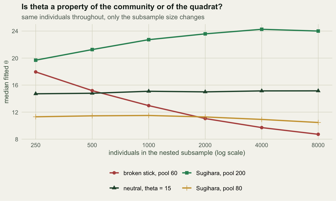
The neutral row is the calibration: fitted \(\theta\) holds flat across a thirty-two-fold change in sample size, ratio 1.00, and the out-of-sample prediction lands -2% from the observed richness. The check passes where it must.
The broken stick row is the check working. A community with a pool of sixty species cannot keep producing new ones, so its fitted \(\theta\) falls by half as the sample grows, ratio 0.49, and the prediction from the small subsample overshoots by +83%: it expects 110 species where 60 exist. That is the diagnostic doing exactly the job it was built for. The Ewens formula has richness growing like \(\theta \log J\) without limit, and every real species pool is finite, so the mismatch is structural rather than statistical.
Check three: what no amount of data will identify
Some things are not a power problem. From the first post, \(\theta = 2 J_M \nu\) enters the likelihood only as a product, so the metacommunity size and the speciation rate are exactly non-identifiable at any sample size, forever. That one needs no simulation; it is visible in the algebra.
Adding \(m\) creates a softer version of the same problem, and softer means it has to be measured rather than read off. Take one simulated plot, move \(\theta\) away from its estimate, reprofile \(m\) at each new value, and see what it costs.
d <- sort(sim_etienne(th0, I0, Jloc), decreasing = TRUE)
LKd <- logK(d, log_stirling1(max(d)))
f0 <- fit2(d, LKd)
prof_m <- function(th) {                                  # the best m for a given theta
  li <- optimize(function(l) -etienne_loglik(d, th, exp(l), LKd), c(log(0.05), log(1e6)))$minimum
  exp(li) / (exp(li) + Jloc - 1)
}
same <- data.frame(theta = f0$theta * c(1, 3, 10, 1000, 1 / 3, 1 / 10))
same$m_profiled <- round(sapply(same$theta, prof_m), 4)
same$logL_drop <- round(mapply(function(th, mm) etienne_loglik(d, th, m_to_I(mm, Jloc), LKd),
                              same$theta, same$m_profiled) - f0$logL, 3)
same$rejected_at_95 <- ifelse(same$logL_drop < -qchisq(0.95, 1) / 2, "yes", "no")
same$theta <- signif(same$theta, 4)
same
theta m_profiled logL_drop rejected_at_95
1 26.040 0.0912 0.000 no
2 78.130 0.0251 -1.017 no
3 260.400 0.0167 -2.726 yes
4 26040.000 0.0140 -3.890 yes
5 8.681 0.9990 -8.885 yes
6 2.604 0.9990 -49.891 yesMultiplying \(\theta\) by three costs 1.02 log-likelihood units against the 1.92 that marks the edge of a 95% interval, and the rejected_at_95 column applies that comparison row by row. Dividing it by three costs 8.88. Across the first two rows \(m\) slides from 0.091 to 0.025 while \(\theta\) triples: a \(\theta\) that can be multiplied while \(m\) takes up the difference is a \(\theta\) the data has not determined. Here the last two rows are pinned against the bound of the search: to explain this plot with a \(\theta\) that small, the model needs every individual to be an immigrant.
This is the same object as the 31% of unbounded intervals from check one, seen from the side. Whenever you see a fitted \(\theta\) with no upper interval limit, this is what produced it, and reporting the point estimate alone hides it completely.
Honest limits
These checks test the sampling formula, not the theory. Etienne, Alonso and McKane (2007) showed that Hubbell’s zero-sum constraint can be dropped without altering the sampling formula. So a plot that passes every check here has told you nothing about zero-sum dynamics, because the formula never encoded them.
Snapshots cannot test dynamics. Neutral theory is a claim about birth, death and dispersal rates being equal across species. Nothing above uses a rate. Repeated censuses of the same plot, which give you turnover, are a different and much sharper instrument, and they are where the theory has actually been in trouble.
The blind spot is a warning about check design, not about these two checks. Both diagnostics here reduce a community to a shape. Adding another that reads the same shape may still raise the catch rate, but on its own such a check is likely to let this community through most of the time too, since the community lands where the neutral shape predicts. What would help is a check that reads something else: spatial arrangement, species identity through time, or trait data. Etienne (2007) took the first of those routes.
Where to go next
If the checking pattern is what you came for rather than neutral theory, the same three moves apply to any fitted model: simulate at a known truth and count coverage, predict something the fit was not shown, and enumerate what the likelihood cannot separate. The other checking posts in this blog run the same routine on different machinery.
References
- Etienne 2005 Ecology Letters 8(3):253-260 (10.1111/j.1461-0248.2004.00717.x)
- Etienne 2007 Ecology Letters 10(7):608-618 (10.1111/j.1461-0248.2007.01052.x)
- Etienne, Alonso & McKane 2007 Journal of Theoretical Biology 248(3):522-536 (10.1016/j.jtbi.2007.06.010)
- Kingman 1978 Journal of the London Mathematical Society s2-18(2):374-380 (10.1112/jlms/s2-18.2.374)
- Chave 2004 Ecology Letters 7(3):241-253 (10.1111/j.1461-0248.2003.00566.x)
- McGill et al 2007 Ecology Letters 10(10):995-1015 (10.1111/j.1461-0248.2007.01094.x)
- Rosindell, Hubbell & Etienne 2011 Trends in Ecology and Evolution 26(7):340-348 (10.1016/j.tree.2011.03.024)