---
title: "Imperfect detection and occupancy bias in R"
description: "Why counting the sites where a species was seen underestimates true occupancy, and how the detection gap grows with fewer survey visits, worked through in R."
date: "2026-07-02 19:00"
categories: [R, occupancy, detection probability, GLM, ecology tutorial]
image: thumbnail.png
image-alt: "Curves showing the share of occupied sites detected at least once, rising with the number of survey visits."
---
```{r}
#| label: setup
#| include: false
suppressMessages({library(ggplot2); library(dplyr); library(tidyr)})
te_ink<-"#16241d"; te_body<-"#2c3a31"; te_forest<-"#275139"; te_paper<-"#f5f4ee"
te_line<-"#dad9ca"; te_faint<-"#5d6b61"; te_gold<-"#c9b458"; te_deep<-"#1d5b4e"
te_red<-"#b5534e"; te_sage<-"#93a87f"; te_green<-"#2f8f63"
theme_te <- function(base_size = 12) {
theme_minimal(base_size = base_size) +
theme(text=element_text(colour=te_body),
plot.title=element_text(colour=te_ink, face="bold", size=rel(1.05)),
plot.subtitle=element_text(colour=te_faint, size=rel(0.9)),
axis.title=element_text(colour=te_ink), axis.text=element_text(colour=te_body),
panel.grid.minor=element_blank(),
panel.grid.major=element_line(colour=te_line, linewidth=0.3),
plot.background=element_rect(fill=te_paper, colour=NA),
panel.background=element_rect(fill=te_paper, colour=NA),
legend.key=element_blank(), legend.position="bottom",
plot.margin=margin(10,12,10,10))
}
```
You survey 200 wetland patches for a frog, hear it at some, and record silence at the rest. The obvious summary is the fraction of patches where you detected it. That number answers a different question from the one you meant to ask. It tells you where the frog was both present and heard, not where it was present. A quiet patch might hold the frog on a night it simply did not call.
This gap between presence and detection is the reason occupancy models exist. Before fitting one, it helps to see exactly how large the bias is, and what drives it. This post builds a landscape where the truth is known, counts what a naive survey would record, and shows that the shortfall follows a simple and predictable rule.
## A landscape where we know the answer
We simulate 200 sites. Each site is truly occupied with probability `psi = 0.55`. At an occupied site, a single visit detects the species with probability `p = 0.30`; an empty site never yields a detection. We visit each site four times.
```{r}
#| label: simulate
set.seed(2026)
R <- 200L; K <- 4L
psi_true <- 0.55; p_true <- 0.30
z <- rbinom(R, 1, psi_true)                                   # true occupancy state
y <- matrix(rbinom(R * K, 1, z * p_true), nrow = R, ncol = K) # detection histories
detected <- rowSums(y)                                        # detections per site (0..4)

sum(z)              # sites truly occupied
mean(z) # realised occupancy
mean(detected >= 1) # naive occupancy: sites detected at least once
```
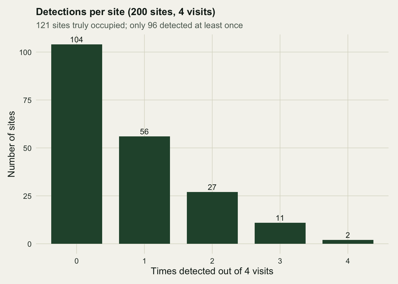
Of the 200 sites, 121 are genuinely occupied, a realised occupancy of 0.605. Yet only 96 sites yield at least one detection across the four visits, so the naive occupancy estimate is 0.48. Roughly a fifth of the occupied sites went unrecorded, and every one of them looks like a true absence in the raw tally.
The full pattern is clearer as a tally of how often each site was detected.
```{r}
#| label: fig-hist
#| fig-cap: "Detections per site across four visits. Sites detected zero times mix genuine absences with occupied sites that were simply missed."
#| fig-alt: "Bar chart of the number of sites by how many times out of four visits the species was detected, with a tall bar at zero."
#| warning: false
hd <- as.data.frame(table(factor(detected, levels = 0:4)))
names(hd) <- c("det", "n")
ggplot(hd, aes(det, n)) +
  geom_col(fill = te_forest, width = 0.75) +
  geom_text(aes(label = n), vjust = -0.4, colour = te_ink, size = 3.5) +
  labs(title = "Detections per site (200 sites, 4 visits)",
       subtitle = "121 sites truly occupied; only 96 detected at least once",
       x = "Times detected out of 4 visits", y = "Number of sites") +
  theme_te(12)
```
The bar at zero is the problem. It holds 104 sites, but only 79 of those are truly empty. The other 25 are occupied sites where four visits all happened to miss the frog.
## The shortfall follows a rule
The size of the gap is not random. A single visit to an occupied site misses the species with probability `1 - p`. Four independent visits all miss it with probability `(1 - p)^4`, so the chance of at least one detection at an occupied site is
$$
P(\text{detected} \mid \text{occupied}) = 1 - (1 - p)^K.
$$
With `p = 0.30` and `K = 4` that probability is `1 - 0.7^4`, which comes to about 0.760. The naive estimate therefore targets `psi` times this fraction, not `psi` itself.
```{r}
#| label: expected
cum_det <- 1 - (1 - p_true)^K          # detection at an occupied site
cum_det                                # about 0.76
psi_true * cum_det # expected naive occupancy
```
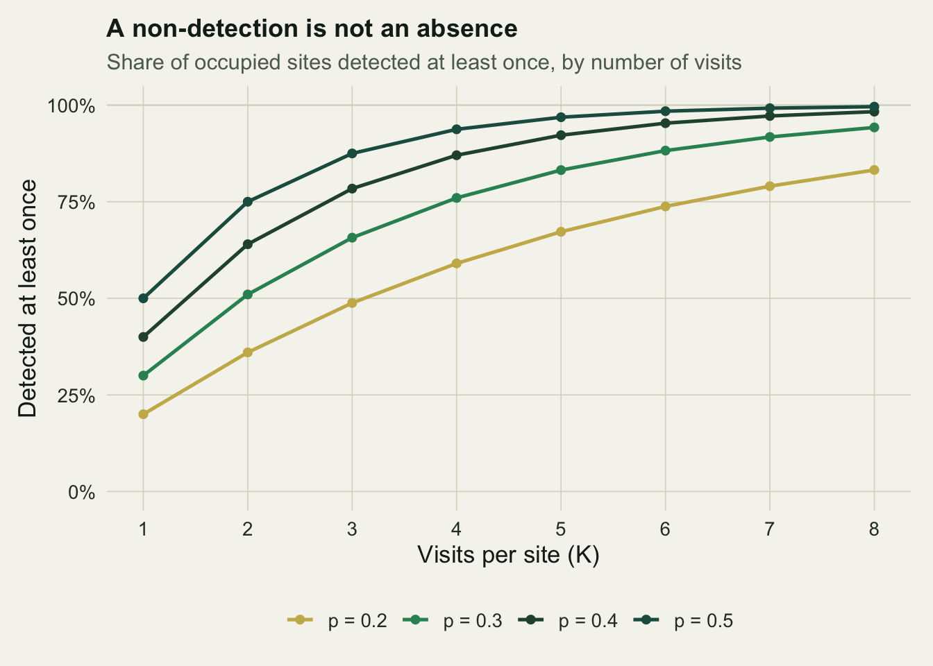
The expected naive occupancy is `0.55 * 0.76`, roughly 0.418, and the value we observed (0.48) sits close to it once sampling noise is allowed for. The ratio of naive to true occupancy is governed entirely by `1 - (1 - p)^K`: raise the detection probability or add visits and the gap shrinks, lower either and it widens. The curve below traces that erosion across a range of detection probabilities.
```{r}
#| label: fig-erosion
#| fig-cap: "Share of occupied sites detected at least once, as a function of visits per site, for four detection probabilities. Low detection needs many visits before a non-detection means much."
#| fig-alt: "Line chart of the probability of at least one detection rising with visits per site, one curve per detection probability, all approaching one."
#| warning: false
K_seq <- 1:8; ps <- c(0.2, 0.3, 0.4, 0.5)
erosion <- expand.grid(K = K_seq, p = ps) |>
  mutate(ratio = 1 - (1 - p)^K, plab = factor(sprintf("p = %.1f", p)))
ggplot(erosion, aes(K, ratio, colour = plab)) +
  geom_hline(yintercept = 1, colour = te_line, linewidth = 0.4) +
  geom_line(linewidth = 0.9) + geom_point(size = 1.7) +
  scale_colour_manual(values = c("p = 0.2"=te_gold, "p = 0.3"=te_green,
                                 "p = 0.4"=te_forest, "p = 0.5"=te_deep), name = NULL) +
  scale_x_continuous(breaks = 1:8) +
  scale_y_continuous(limits = c(0, 1), labels = scales::percent_format(1)) +
  labs(title = "A non-detection is not an absence",
       subtitle = "Share of occupied sites detected at least once, by number of visits",
       x = "Visits per site (K)", y = "Detected at least once") +
  theme_te(13)
```
At `p = 0.3`, a single visit finds only a third of occupied sites, and it takes around eight visits before you would expect to detect nearly all of them. A rare or quiet species at the low end of the chart can be badly under-recorded even after a full field season.
## The detection rate is biased too
The trouble does not stop at occupancy. Suppose you tried to estimate `p` itself from the raw data by taking the average detection rate among sites where the species was found. Conditioning on at least one detection throws away the zeros that belong to occupied sites, so the surviving sites are the ones where detection happened to run high.
```{r}
#| label: phat-naive
det_sites <- detected[detected >= 1]
mean(det_sites) / K   # naive detection rate among detected sites
```
The naive figure is 0.393, well above the true 0.30. Both quantities you care about, how widespread the species is and how detectable it is, are distorted when non-detections are read as absences. The two biases are linked: pretend detection is perfect and you must also pretend every silent site is empty.
## Real surveys behave this way
This is not a quirk of simulated data. In the study that introduced the single-season occupancy model, MacKenzie and colleagues re-analysed anuran calling surveys and found that accounting for imperfect detection raised the occupancy estimate for one species to 0.49, a 44 per cent increase over the proportion of sites where it was actually recorded. The raw proportion had been treating missed calls as true absences, exactly as our tally does.
## Where this leads
The fix is not to visit every site until you are certain, which is rarely affordable. It is to use the repeat visits you already have. The pattern of detections and non-detections across visits carries information about both `psi` and `p`, and a likelihood written around `1 - (1 - p)^K` can separate them. The next tutorial fits that model to this very dataset and recovers an occupancy estimate close to the true 0.55, rather than the biased 0.48 the raw counts gave.
## References
- MacKenzie D I, Nichols J D, Lachman G B, Droege S, Royle J A, Langtimm C A 2002 Ecology 83(8):2248-2255 (10.1890/0012-9658(2002)083[2248:ESORWD]2.0.CO;2)
- Tyre A J, Tenhumberg B, Field S A, Niejalke D, Parris K, Possingham H P 2003 Ecological Applications 13(6):1790-1801 (10.1890/02-5078)
## Related tutorials
- [Fitting single-season occupancy models in R](../single-season-occupancy-model/)
- [How many visits? Occupancy survey design](../survey-design-detection-visits/)
- [Logistic regression for presence/absence data](../logistic-regression-presence-absence/)
- [Species distribution modelling with GLM in R](../species-distribution-model-glm/)