---
title: "Fitting single-season occupancy models in R"
description: "Build the MacKenzie occupancy likelihood from scratch and fit it with optim to separate true site occupancy from detection probability, using base R only."
date: "2026-07-02 20:00"
categories: [R, occupancy, maximum likelihood, detection probability, ecology tutorial]
image: thumbnail.png
image-alt: "Point-range chart comparing naive occupancy, the occupancy-model estimate with confidence interval, and true occupancy."
---
```{r}
#| label: setup
#| include: false
suppressMessages({library(ggplot2)})
te_ink<-"#16241d"; te_body<-"#2c3a31"; te_forest<-"#275139"; te_paper<-"#f5f4ee"
te_line<-"#dad9ca"; te_faint<-"#5d6b61"; te_gold<-"#c9b458"; te_deep<-"#1d5b4e"
te_red<-"#b5534e"; te_sage<-"#93a87f"; te_green<-"#2f8f63"
theme_te <- function(base_size = 12) {
theme_minimal(base_size = base_size) +
theme(text=element_text(colour=te_body),
plot.title=element_text(colour=te_ink, face="bold", size=rel(1.05)),
plot.subtitle=element_text(colour=te_faint, size=rel(0.9)),
axis.title=element_text(colour=te_ink), axis.text=element_text(colour=te_body),
panel.grid.minor=element_blank(),
panel.grid.major=element_line(colour=te_line, linewidth=0.3),
plot.background=element_rect(fill=te_paper, colour=NA),
panel.background=element_rect(fill=te_paper, colour=NA),
legend.key=element_blank(), legend.position="bottom",
plot.margin=margin(10,12,10,10))
}
```
A companion tutorial showed that counting the sites where a species was detected underestimates how widespread it is, because a quiet site looks the same as an empty one. The repeat visits you make to each site are what rescue the estimate: the sequence of detections and blanks across visits tells you how often the species is missed, and from that you can back out how many silent sites were occupied all along.
This post writes the single-season occupancy likelihood by hand and fits it with `optim`. No specialised package is needed. Working through the likelihood makes clear what the model assumes and why it can separate occupancy from detection at all.
## The same simulated data
We reuse the landscape from the detection-bias tutorial: 200 sites, true occupancy `psi = 0.55`, per-visit detection `p = 0.30`, four visits each. Naive occupancy came out at 0.48 against a realised truth of 0.605.
```{r}
#| label: data
set.seed(2026)
R <- 200L; K <- 4L; psi_true <- 0.55; p_true <- 0.30
z <- rbinom(R, 1, psi_true)
y <- matrix(rbinom(R * K, 1, z * p_true), nrow = R, ncol = K)
d <- rowSums(y)                # detections per site
mean(d >= 1)                   # naive occupancy
```
## The likelihood, site by site
Each site contributes one term to the likelihood, and there are only two cases.
If a site was detected on at least one visit, it must be occupied. The probability of its exact history is the occupancy probability times the detection pattern: `psi` for being occupied, `p` for each of the `d` visits with a detection, and `1 - p` for each of the `K - d` visits without one. That gives
$$
L_i = \psi \, p^{\,d_i} (1 - p)^{\,K - d_i}, \qquad d_i \ge 1.
$$
If a site was never detected across all `K` visits, two explanations remain. Either it is occupied and every visit missed the species, with probability `psi (1 - p)^K`, or it is genuinely empty, with probability `1 - psi`. Since both would produce an all-blank history, the term is their sum:
$$
L_i = \psi (1 - p)^K + (1 - \psi), \qquad d_i = 0.
$$
That second line is where the model earns its keep. The all-blank sites are a mixture of missed occupancy and true absence, and the relative weight of the two is pinned down by how detectable the species proves to be at the sites where it was seen. A species detected on most visits leaves few plausible misses, so most blanks are real absences; a rarely detected species leaves room for many occupied blanks.
We estimate on the logit scale so the optimiser can range over the whole real line while `psi` and `p` stay inside zero and one.
```{r}
#| label: nll
nll <- function(par, y, K) {
  psi <- plogis(par[1]); p <- plogis(par[2])
  d <- rowSums(y)
  lik <- ifelse(d > 0,
                psi * p^d * (1 - p)^(K - d),
                psi * (1 - p)^K + (1 - psi))
  -sum(log(lik))
}
fit <- optim(c(0, 0), nll, y = y, K = K, method = "BFGS", hessian = TRUE)
psi_hat <- plogis(fit$par[1])
p_hat   <- plogis(fit$par[2])
c(psi_hat = round(psi_hat, 3), p_hat = round(p_hat, 3))
```
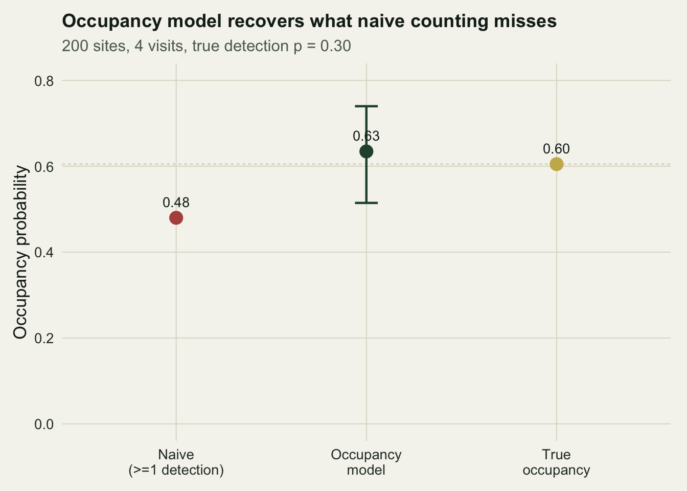
The model recovers `psi_hat = 0.635` and `p_hat = 0.297`. The occupancy estimate has moved from the naive 0.48 up towards the realised 0.605, and the detection estimate sits almost exactly on the true 0.30, rather than the inflated 0.393 the raw detected-site average gave. The figure below places the three occupancy numbers side by side.
```{r}
#| label: fig-compare
#| fig-cap: "Naive occupancy, the occupancy-model estimate with its 95 per cent interval, and the realised true occupancy. The model closes most of the gap the naive count leaves open."
#| fig-alt: "Point-range chart with naive occupancy well below true occupancy and the model estimate close to truth with a confidence interval spanning it."
#| warning: false
V <- solve(fit$hessian); sl <- sqrt(diag(V))
psi_ci <- plogis(fit$par[1] + c(-1.96, 1.96) * sl[1])
est <- data.frame(
  what = factor(c("Naive\n(>=1 detection)", "Occupancy\nmodel", "True\noccupancy"),
                levels = c("Naive\n(>=1 detection)", "Occupancy\nmodel", "True\noccupancy")),
  val  = c(mean(d >= 1), psi_hat, mean(z)),
  lo   = c(NA, psi_ci[1], NA), hi = c(NA, psi_ci[2], NA),
  kind = c("naive", "model", "truth"))
ggplot(est, aes(what, val, colour = kind)) +
  geom_hline(yintercept = mean(z), colour = te_line, linewidth = 0.5, linetype = "22") +
  geom_errorbar(aes(ymin = lo, ymax = hi), width = 0.12, linewidth = 0.8, na.rm = TRUE) +
  geom_point(size = 4) +
  geom_text(aes(label = sprintf("%.2f", val)), vjust = -1.1, size = 3.6, colour = te_ink) +
  scale_colour_manual(values = c(naive = te_red, model = te_forest, truth = te_gold), guide = "none") +
  scale_y_continuous(limits = c(0, 0.8)) +
  labs(title = "Occupancy model recovers what naive counting misses",
       subtitle = "200 sites, 4 visits, true detection p = 0.30",
       x = NULL, y = "Occupancy probability") +
  theme_te(13)
```
## How precise is the estimate?
The Hessian that `optim` returns is the curvature of the negative log-likelihood at its minimum, so its inverse is the covariance of the parameters on the logit scale. To report a standard error on the probability scale, transform the logit-scale error with the delta method: the derivative of `plogis` at a point equals the fitted probability times one minus itself.
```{r}
#| label: se
se_logit <- sqrt(diag(V))
se_psi <- se_logit[1] * psi_hat * (1 - psi_hat)
se_p   <- se_logit[2] * p_hat   * (1 - p_hat)
round(c(se_psi = se_psi, se_p = se_p), 3)
plogis(fit$par[1] + c(-1.96, 1.96) * se_logit[1]) # 95% CI for psi
plogis(fit$par[2] + c(-1.96, 1.96) * se_logit[2]) # 95% CI for p
```
Occupancy carries a standard error of 0.058, with a 95 per cent interval of about 0.515 to 0.740, so the true 0.55 sits comfortably inside it. Detection is pinned down more tightly, at 0.297 with an interval of 0.242 to 0.360. Note that building the interval on the logit scale and then transforming keeps it inside zero and one, which a plain estimate plus or minus two standard errors would not guarantee near the boundary.
## The surface being climbed
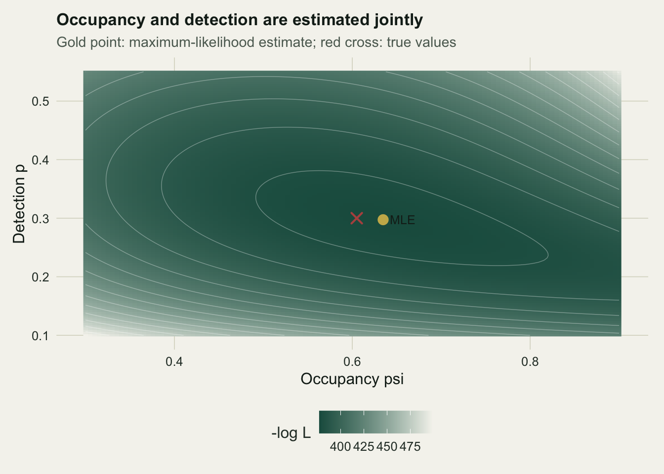
It helps to see what `optim` is doing. The negative log-likelihood is a surface over the two parameters, and the fit is its lowest point. Evaluating it across a grid shows a single well, with the maximum-likelihood estimate at the bottom and the true values close by.
```{r}
#| label: fig-surface
#| fig-cap: "The negative log-likelihood over occupancy and detection. The gold point is the maximum-likelihood estimate; the red cross marks the true values used to simulate the data."
#| fig-alt: "Filled contour surface over occupancy and detection probability with a single minimum, marked by a point near a cross for the true values."
#| warning: false
#| message: false
gp <- seq(0.30, 0.90, length.out = 120); gq <- seq(0.10, 0.55, length.out = 120)
Z <- outer(gp, gq, Vectorize(function(P, Q) nll(c(qlogis(P), qlogis(Q)), y, K)))
dfz <- expand.grid(psi = gp, p = gq); dfz$nll <- as.vector(Z)
ggplot(dfz, aes(psi, p, z = nll)) +
  geom_raster(aes(fill = nll)) +
  geom_contour(colour = "#ffffff", alpha = 0.35, linewidth = 0.25, bins = 14) +
  scale_fill_gradient(low = te_deep, high = te_paper, name = "-log L") +
  annotate("point", x = psi_hat, y = p_hat, colour = te_gold, size = 3.2) +
  annotate("point", x = mean(z), y = p_true, colour = te_red, shape = 4, size = 3, stroke = 1.1) +
  annotate("text", x = psi_hat, y = p_hat, label = "  MLE", hjust = 0, colour = te_ink, size = 3.3) +
  labs(title = "Occupancy and detection are estimated jointly",
       subtitle = "Gold point: maximum-likelihood estimate; red cross: true values",
       x = "Occupancy psi", y = "Detection p") +
  theme_te(12)
```
## More visits, sharper separation
The single dataset gives one draw of the estimator. The precision improves as visits accumulate, because more visits pin down `p`, and a well-estimated `p` leaves less ambiguity about the all-blank sites. Refitting with eight visits instead of four narrows the occupancy standard error markedly.
```{r}
#| label: k8
set.seed(2026)
K8 <- 8L
z8 <- rbinom(R, 1, psi_true)
y8 <- matrix(rbinom(R * K8, 1, z8 * p_true), R, K8)
fit8 <- optim(c(0, 0), nll, y = y8, K = K8, method = "BFGS", hessian = TRUE)
se8 <- sqrt(diag(solve(fit8$hessian)))[1] * plogis(fit8$par[1]) * (1 - plogis(fit8$par[1]))
c(psi_hat = round(plogis(fit8$par[1]), 3),
  p_hat   = round(plogis(fit8$par[2]), 3),
  se_psi  = round(se8, 3))
```
With eight visits the occupancy estimate is 0.609 with a standard error of 0.037, down from 0.058 at four visits. How to trade the number of sites against the number of visits under a fixed budget is a design question in its own right, taken up in a later tutorial.
## What the model assumes
The likelihood leans on a few conditions worth stating plainly. Occupancy is treated as fixed across the visit window, so the site does not gain or lose the species between visits, which is what single-season means. Detection is assumed independent across visits given occupancy, and false detections are ruled out, so a recorded detection is never a mistake. When those hold, the repeat-visit structure identifies `psi` and `p` separately. When they do not, for instance if the species arrives partway through the season, the estimates shift, and a dynamic or multi-season model becomes the honest choice.
The next step is to let occupancy and detection depend on covariates, so that `psi` can vary with habitat and `p` with survey effort, which is where the model becomes useful for real questions.
## References
- MacKenzie D I, Nichols J D, Lachman G B, Droege S, Royle J A, Langtimm C A 2002 Ecology 83(8):2248-2255 (10.1890/0012-9658(2002)083[2248:ESORWD]2.0.CO;2)
- MacKenzie D I, Nichols J D, Royle J A, Pollock K H, Bailey L L, Hines J E 2018 Occupancy Estimation and Modeling, 2nd ed. Academic Press. ISBN 978-0-12-407197-1
- Fiske I, Chandler R B 2011 Journal of Statistical Software 43(10):1-23 (10.18637/jss.v043.i10)
## Related tutorials
- [Imperfect detection and occupancy bias in R](../imperfect-detection-occupancy/)
- [Occupancy and detection covariates in R](../occupancy-detection-covariates/)
- [Logistic regression for presence/absence data](../logistic-regression-presence-absence/)
- [N-mixture models for abundance in R](../n-mixture-models-abundance/)